Characterization of the employment demand and registered contracting in Spain


Fecha del documento: 13-09-2021

1. Introduction
Data visualization is a task linked to data analysis that aims to represent graphically the underlying information. Visualizations play a fundamental role in data communication, since they allow to draw conclusions in a visual and understandable way, also allowing detection of patterns, trends, anomalous data or projection of predictions, among many other functions. This makes its application transversal to any process that involves data. The visualization possibilities are very broad, from basic representations such as line, bar or sector graph, to complex visualizations configured on interactive dashboards.
Before starting to build an effective visualization, a prior data treatment must be performed, paying attention to their collection and validation of their content, ensuring that they are free of errors and in an adequate and consistent format for processing. The previous data treatment is essential to carry out any task related to data analysis and realization of effective visualizations.
We will periodically present a series of practical exercises on open data visualizations that are available on the portal datos.gob.es and in other similar catalogues. In there, we approach and describe in a simple way the necessary steps to obtain data, perform transformations and analysis that are relevant to creation of interactive visualizations from which we may extract all the possible information summarised in final conclusions. In each of these practical exercises we will use simple code developments which will be conveniently documented, relying on free tools. Created material will be available to reuse in Data Lab on Github.
Captura del vídeo que muestra la interacción con el dashboard de la caracterización de la demanda de empleo y la contratación registrada en España disponible al final de este artículo
2. Objetives
The main objective of this post is to create an interactive visualization using open data. For this purpose, we have used datasets containing relevant information on evolution of employment demand in Spain over the last years. Based on these data, we have determined a profile that represents employment demand in our country, specifically investigating how does gender gap affects a group and impact of variables such as age, unemployment benefits or region.
3. Resources
3.1. Datasets
For this analysis we have selected datasets published by the Public State Employment Service (SEPE), coordinated by the Ministry of Labour and Social Economy, which collects time series data with distinct breakdowns that facilitate the analysis of the qualities of job seekers. These data are available on datos.gob.es, with the following characteristics:
- Demandantes de empleo por municipio: contains the number of job seekers broken down by municipality, age and gender, between the years 2006-2020.
- Gasto de prestaciones por desempleo por Provincia: time series between the years 2010-2020 related to unemployment benefits expenditure, broken down by province and type of benefit.
- Contratos registrados por el Servicio Público de Empleo Estatal (SEPE) por municipio: these datasets contain the number of registered contracts to both, job seekers and non-job seekers, broken down by municipality, gender and contract type, between the years 2006-2020.
3.2. Tools.
R (versión 4.0.3) and RStudio with RMarkdown add-on have been used to carry out this analysis (working environment, programming and drafting).
RStudio is an integrated open source development environment for R programming language, dedicated to statistical analysis and graphs creation.
RMarkdown allows creation of reports integrating text, code and dynamic results into a single document.
To create interactive graphs, we have used Kibana tool.
Kibana is an open code application that forms a part of Elastic Stack (Elasticsearch, Beats, Logstasg y Kibana) qwhich provides visualization and exploration capacities of the data indexed on the analytics engine Elasticsearch. The main advantages of this tool are:
- Presents visual information through interactive and customisable dashboards using time intervals, filters faceted by range, geospatial coverage, among others
- Contains development tools catalogue (Dev Tools) to interact with data stored in Elasticsearch.
- It has a free version ready to use on your own computer and enterprise version that is developed in the Elastic cloud and other cloud infrastructures, such as Amazon Web Service (AWS).
On Elastic website you may find user manuals for the download and installation of the tool, but also how to create graphs, dashboards, etc. Furthermore, it offers short videos on the youtube channel and organizes webinars dedicated to explanation of diverse aspects related to Elastic Stack.
If you want to learn more about these and other tools which may help you with data processing, see the report “Data processing and visualization tools” that has been recently updated.
4. Data processing
To create a visualization, it´s necessary to prepare the data properly by performing a series of tasks that include pre-processing and exploratory data analysis (EDA), to understand better the data that we are dealing with. The objective is to identify data characteristics and detect possible anomalies or errors that could affect the quality of results. Data pre-processing is essential to ensure the consistency and effectiveness of analysis or visualizations that are created afterwards.
In order to support learning of readers who are not specialised in programming, the R code included below, which can be accessed by clicking on “Code” button, is not designed to be efficient but rather to be easy to understand. Therefore, it´s probable that the readers more advanced in this programming language may consider to code some of the functionalities in an alternative way. A reader will be able to reproduce this analysis if desired, as the source code is available on the datos.gob.es Github account. The way to provide the code is through a RMarkdown document. Once it´s loaded to the development environment, it may be easily run or modified.
4.1. Installation and import of libraries
R base package, which is always available when RStudio console is open, includes a wide set of functionalities to import data from external sources, carry out statistical analysis and obtain graphic representations. However, there are many tasks for which it´s required to resort to additional packages, incorporating functions and objects defined in them into the working environment. Some of them are already available in the system, but others should be downloaded and installed.
4.2. Data import and cleansing
a. Import of datasets
Data which will be used for visualization are divided by annualities in the .CSV and .XLS files. All the files of interest should be imported to the development environment. To make this post easier to understand, the following code shows the upload of a single .CSV file into a data table.
To speed up the loading process in the development environment, it´s necessary to download the datasets required for this visualization to the working directory. The datasets are available on the datos.gob.es Github account.
Once all the datasets are uploaded as data tables in the development environment, they need to be merged in order to obtain a single dataset that includes all the years of the time series, for each of the characteristics related to job seekers that will be analysed: number of job seekers, unemployment expenditure and new contracts registered by SEPE.
b. Selection of variables
Once the tables with three time series are obtained (number of job seekers, unemployment expenditure and new registered contracts), the variables of interest will be extracted and included in a new table.
First, the tables with job seekers (“unemployment_data”) and new registered contracts (“contracts”) should be added by province, to facilitate the visualization. They should match the breakdown by province of the unemployment benefits expenditure table (“unemployment_expentidure”). In this step, only the variables of interest will be selected from the three datasets.
Secondly, the three tables should be merged into one that we will work with from this point onwards..
c. Transformation of variables
When the table with variables of interest is created for further analysis and visualization, some of them should be transformed to other types, more adequate for future aggregations.
d. Exploratory analysis
Let´s see what variables and structure the new dataset presents.
The output of this portion of the code is omitted to facilitate reading. Main characteristics presented in the dataset are as follows:
- Time range covers a period from January to December 2020.
- Number of columns (variables) is 17. .
- It presents two categorical variables (“Province”, “Autonomous.Community”), one date variable (“Code.month”) and the rest are numerical variables.
e. Detection and processing of missing data
Next, we will analyse whether the dataset has missing values (NAs). A treatment or elimination of NAs is essential, otherwise it will not be possible to process properly the numerical variables.
4.3. Creation of new variables
In order to create a visualization, we are going to make a new variable from the two variables present in the data table. This operation is very common in the data analysis, as sometimes it´s interesting to work with calculated data (e.g., the sum or the average of different variables) instead of source data. In this case, we will calculate the average unemployment expenditure for each job seeker. For this purpose, variables of total expenditure per benefit (“Expenditure.Total.Benefit”) and the total number of job seekers (“total.JobSeekers.Employment”) will be used.
4.4. Save the dataset
Once the table containing variables of interest for analysis and visualizations is obtained, we will save it as a data file in CSV format to perform later other statistical analysis or use it within other processing or data visualization tools. It´s important to use the UTF-8 encoding (Unicode Transformation Format), so the special characters may be identified correctly by any other tool.
5. Creation of a visualization on the characteristics of employment demand in Spain using Kibana
The development of this interactive visualization has been performed with usage of Kibana in the local environment. We have followed Elastic company tutorial for both, download and installation of the software.
Below you may find a tutorial video related to the whole process of creating a visualization. In the video you may see the creation of dashboard with different interactive indicators by generating graphic representations of different types. The steps to build a dashboard are as follows:
A continuación se adjunta un vídeo tutorial donde se muestra todo el proceso de realización de la visualización. En el vídeo podrás ver la creación de un cuadro de mando (dashboard) con diferentes indicadores interactivos mediante la generación de representaciones gráficas de diferentes tipos. Los pasos para obtener el dashboard son los siguientes:
- Load the data into Elasticsearch and generate an index that allows to interact with the data from Kibana. This index permits a search and management of the data in the loaded files, practically in real time.
- Generate the following graphic representations:
- Line graph to represent a time series on the job seekers in Spain between 2006 and 2020.
- Sector graph with job seekers broken down by province and Autonomous Community
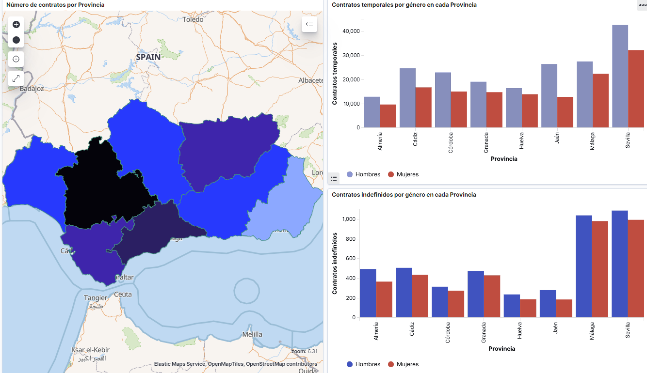
- Thematic map showing the number of new contracts registered in each province on the territory. For creation of this visual it´s necessary to download a dataset with province georeferencing published in the open data portal Open Data Soft.
- Build a dashboard.
Below you may find a tutorial video interacting with the visualization that we have just created:
6. Conclusions
Looking at the visualization of the data related to the profile of job seekers in Spain during the years 2010-2020, the following conclusions may be drawn, among others:
- There are two significant increases of the job seekers number. The first, approximately in 2010, coincides with the economic crisis. The second, much more pronounced in 2020, coincides with the pandemic crisis.
- A gender gap may be observed in the group of job seekers: the number of female job seekers is higher throughout the time series, mainly in the age groups above 25.
- At the regional level, Andalusia, followed by Catalonia and Valencia, are the Autonomous Communities with the highest number of job seekers. In contrast to Andalusia, which is an Autonomous Community with the lowest unemployment expenditure, Catalonia presents the highest value.
- Temporal contracts are leading and the provinces which generate the highest number of contracts are Madrid and Barcelona, what coincides with the highest number of habitants, while on the other side, provinces with the lowest number of contracts are Soria, Ávila, Teruel and Cuenca, what coincides with the most depopulated areas of Spain.
This visualization has helped us to synthetise a large amount of information and give it a meaning, allowing to draw conclusions and, if necessary, make decisions based on results. We hope that you like this new post, we will be back to present you new reuses of open data. See you soon!