Blog
In this post we have described step-by-step a data science exercise in which we try to train a deep learning model with a view to automatically classifying medical images of healthy and sick people.
Diagnostic imaging has been around for many years in the hospitals of developed countries; however, there has always been a strong dependence on highly specialised personnel. From the technician who operates the instruments to the radiologist who interprets the images. With our current analytical capabilities, we are able to extract numerical measures such as volume, dimension, shape and growth rate (inter alia) from image analysis. Throughout this post we will try to explain, through a simple example, the power of artificial intelligence models to expand human capabilities in the field of medicine.
This post explains the practical exercise (Action section) associated with the report “Emerging technologies and open data: introduction to data science applied to image analysis”. Said report introduces the fundamental concepts that allow us to understand how image analysis works, detailing the main application cases in various sectors and highlighting the role of open data in their implementation.
Previous projects
However, we could not have prepared this exercise without the prior work and effort of other data science lovers. Below we have provided you with a short note and the references to these previous works.
- This exercise is an adaptation of the original project by Michael Blum on the STOIC2021 - disease-19 AI challenge. Michael's original project was based on a set of images of patients with Covid-19 pathology, along with other healthy patients to serve as a comparison.
- In a second approach, Olivier Gimenez used a data set similar to that of the original project published in a competition of Kaggle. This new dataset (250 MB) was considerably more manageable than the original one (280GB). The new dataset contained just over 1,000 images of healthy and sick patients. Olivier's project code can be found at the following repository.
Datasets
In our case, inspired by these two amazing previous projects, we have built an educational exercise based on a series of tools that facilitate the execution of the code and the possibility of examining the results in a simple way. The original data set (chest x-ray) comprises 112,120 x-ray images (front view) from 30,805 unique patients. The images are accompanied by the associated labels of fourteen diseases (where each image can have multiple labels), extracted from associated radiological reports using natural language processing (NLP). From the original set of medical images we have extracted (using some scripts) a smaller, delimited sample (only healthy people compared with people with just one pathology) to facilitate this exercise. In particular, the chosen pathology is pneumothorax.
If you want further information about the field of natural language processing, you can consult the following report which we already published at the time. Also, in the post 10 public data repositories related to health and wellness the NIH is referred to as an example of a source of quality health data. In particular, our data set is publicly available here.
Tools
To carry out the prior processing of the data (work environment, programming and drafting thereof), R (version 4.1.2) and RStudio (2022-02-3) was used. The small scripts to help download and sort files have been written in Python 3.
Accompanying this post, we have created a Jupyter notebook with which to experiment interactively through the different code snippets that our example develops. The purpose of this exercise is to train an algorithm to be able to automatically classify a chest X-ray image into two categories (sick person vs. non-sick person). To facilitate the carrying out of the exercise by readers who so wish, we have prepared the Jupyter notebook in the Google Colab environment which contains all the necessary elements to reproduce the exercise step-by-step. Google Colab or Collaboratory is a free Google tool that allows you to programme and run code on python (and also in R) without the need to install any additional software. It is an online service and to use it you only need to have a Google account.
Logical flow of data analysis
Our Jupyter Notebook carries out the following differentiated activities which you can follow in the interactive document itself when you run it on Google Colab.
- Installing and loading dependencies.
- Setting up the work environment
- Downloading, uploading and pre-processing of the necessary data (medical images) in the work environment.
- Pre-visualisation of the loaded images.
- Data preparation for algorithm training.
- Model training and results.
- Conclusions of the exercise.
Then we carry out didactic review of the exercise, focusing our explanations on those activities that are most relevant to the data analysis exercise:
- Description of data analysis and model training
- Modelling: creating the set of training images and model training
- Analysis of the training result
- Conclusions
Description of data analysis and model training
The first steps that we will find going through the Jupyter notebook are the activities prior to the image analysis itself. As in all data analysis processes, it is necessary to prepare the work environment and load the necessary libraries (dependencies) to execute the different analysis functions. The most representative R package of this set of dependencies is Keras. In this article we have already commented on the use of Keras as a Deep Learning framework. Additionally, the following packages are also required: htr; tidyverse; reshape2; patchwork.
Then we have to download to our environment the set of images (data) we are going to work with. As we have previously commented, the images are in remote storage and we only download them to Colab at the time we analyse them. After executing the code sections that download and unzip the work files containing the medical images, we will find two folders (No-finding and Pneumothorax) that contain the work data.

Once we have the work data in Colab, we must load them into the memory of the execution environment. To this end, we have created a function that you will see in the notebook called process_pix(). This function will search for the images in the previous folders and load them into the memory, in addition to converting them to grayscale and normalising them all to a size of 100x100 pixels. In order not to exceed the resources that Google Colab provides us with for free, we limit the number of images that we load into memory to 1000 units. In other words, the algorithm will be trained with 1000 images, including those that it will use for training and those that it will use for subsequent validation.
Once we have the images perfectly classified, formatted and loaded into memory, we carry out a quick visualisation to verify that they are correct. We obtain the following results:

Self-evidently, in the eyes of a non-expert observer, there are no significant differences that allow us to draw any conclusions. In the steps below we will see how the artificial intelligence model actually has a better clinical eye than we do.
Modelling
Creating the training image set
As we mentioned in the previous steps, we have a set of 1000 starting images loaded in the work environment. Until now, we have had classified (by an x-ray specialist) those images of patients with signs of pneumothorax (on the path "./data/Pneumothorax") and those patients who are healthy (on the path "./data/No -Finding")
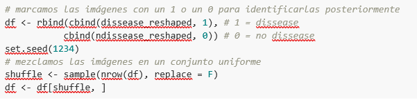
The aim of this exercise is precisely to demonstrate the capacity of an algorithm to assist the specialist in the classification (or detection of signs of disease in the x-ray image). With this in mind, we have to mix the images to achieve a homogeneous set that the algorithm will have to analyse and classify using only their characteristics. The following code snippet associates an identifier (1 for sick people and 0 for healthy people) so that, later, after the algorithm's classification process, it is possible to verify those that the model has classified correctly or incorrectly.
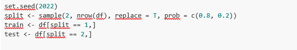
So, now we have a uniform “df” set of 1000 images mixed with healthy and sick patients. Next, we split this original set into two. We are going to use 80% of the original set to train the model. In other words, the algorithm will use the characteristics of the images to create a model that allows us to conclude whether an image matches the identifier 1 or 0. On the other hand, we are going to use the remaining 20% of the homogeneous mixture to check whether the model, once trained, is capable of taking any image and assigning it 1 or 0 (sick, not sick).
Model training
Right, now all we have left to do is to configure the model and train with the previous data set.
Before training, you will see some code snippets which are used to configure the model that we are going to train. The model we are going to train is of the binary classifier type. This means that it is a model that is capable of classifying the data (in our case, images) into two categories (in our case, healthy or sick). The model selected is called CNN or Convolutional Neural Network. Its very name already tells us that it is a neural networks model and thus falls under the Deep Learning discipline. These models are based on layers of data features that get deeper as the complexity of the model increases. We would remind you that the term deep refers precisely to the depth of the number of layers through which these models learn.
Note: the following code snippets are the most technical in the post. Introductory documentation can be found here, whilst all the technical documentation on the model's functions is accessible here.
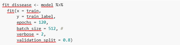
Finally, after configuring the model, we are ready to train the model. As we mentioned, we train with 80% of the images and validate the result with the remaining 20%.
Training result
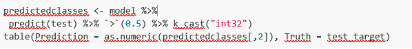
Well, now we have trained our model. So what's next? The graphs below provide us with a quick visualisation of how the model behaves on the images that we have reserved for validation. Basically, these figures actually represent (the one in the lower panel) the capability of the model to predict the presence (identifier 1) or absence (identifier 0) of disease (in our case pneumothorax). The conclusion is that when the model trained with the training images (those for which the result 1 or 0 is known) is applied to 20% of the images for which the result is not known, the model is correct approximately 85% (0.87309) of times.

Indeed, when we request the evaluation of the model to know how well it classifies diseases, the result indicates the capability of our newly trained model to correctly classify 0.87309 of the validation images.
Now let’s make some predictions about patient images. In other words, once the model has been trained and validated, we wonder how it is going to classify the images that we are going to give it now. As we know "the truth" (what is called the ground truth) about the images, we compare the result of the prediction with the truth. To check the results of the prediction (which will vary depending on the number of images used in the training) we use that which in data science is called the confusion matrix. The confusion matrix:
- Places in position (1,1) the cases that DID have disease and the model classifies as "with disease"
- Places in position (2,2), the cases that did NOT have disease and the model classifies as "without disease"
In other words, these are the positions in which the model "hits" its classification.
In the opposite positions, in other words, (1,2) and (2,1) are the positions in which the model is "wrong". So, position (1,2) are the results that the model classifies as WITH disease and the reality is that they were healthy patients. Position (2,1), the very opposite.
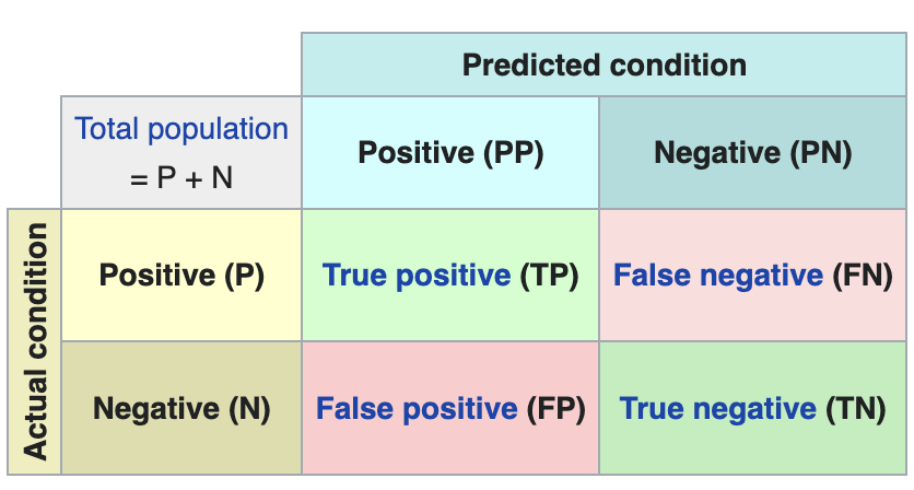
Explanatory example of how the confusion matrix works. Source: Wikipedia https://en.wikipedia.org/wiki/Confusion_matrix
In our exercise, the model gives us the following results:
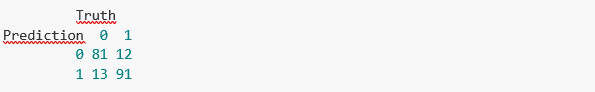
In other words, 81 patients had this disease and the model classifies them correctly. Similarly, 91 patients were healthy and the model also classifies them correctly. However, the model classifies as sick 13 patients who were healthy. Conversely, the model classifies 12 patients who were actually sick as healthy. When we add the hits of the 81+91 model and divide it by the total validation sample, we obtain 87% accuracy of the model.
Conclusions
In this post we have guided you through a didactic exercise consisting of training an artificial intelligence model to carry out chest x-ray imaging classifications with the aim of determining automatically whether someone is sick or healthy. For the sake of simplicity, we have chosen healthy patients and patients with pneumothorax (only two categories) previously diagnosed by a doctor. The journey we have taken gives us an insight into the activities and technologies involved in automated image analysis using artificial intelligence. The result of the training affords us a reasonable classification system for automatic screening with 87% accuracy in its results. Algorithms and advanced image analysis technologies are, and will increasingly be, an indispensable complement in multiple fields and sectors, such as medicine. In the coming years, we will see the consolidation of systems which naturally combine the skills of humans and machines in expensive, complex or dangerous processes. Doctors and other workers will see their capabilities increased and strengthened thanks to artificial intelligence. The joining of forces between machines and humans will allow us to reach levels of precision and efficiency never seen before. We hope that through this exercise we have helped you to understand a little more about how these technologies work. Don't forget to complete your learning with the rest of the materials that accompany this post.
Content prepared by Alejandro Alija, an expert in Digital Transformation.The contents and points of view reflected in this publication are the sole responsibility of its author.
Blog
The democratisation of technology in all areas is an unstoppable trend. With the spread of smartphones and Internet access, an increasing number of people can access high-tech products and services without having to resort to advanced knowledge or specialists. The world of data is no stranger to this transformation and in this post we tell you why.
Introduction
Nowadays, you don't need to be an expert in video editing and post-production to have your own YouTube channel and generate high quality content. In the same way that you don't need to be a super specialist to have a smart and connected home. This is due to the fact that technology creators are paying more and more attention to providing simple tools with a careful user experience for the average consumer. It is a similar story with data. Given the importance of data in today's society, both for private and professional use, in recent years we have seen the democratisation of tools for simple data analysis, without the need for advanced programming skills.
In this sense, spreadsheets have always lived among us and we have become so accustomed to their use that we use them for almost anything, from a shopping list to a family budget. Spreadsheets are so popular that they are even considered as a sporting event. However, despite their great versatility, they are not the most visual tools from the point of view of communicating information. Moreover, spreadsheets are not suitable for a type of data that is becoming more and more important nowadays: real-time data.
The natively digital world increasingly generates real-time data. Some reports suggest that by 2025, a quarter of the world's data will be real-time data. That is, it will be data with a much shorter lifecycle, during which it will be generated, analysed in real time and disappear as it will not make sense to store it for later use. One of the biggest contributors to real-time data will be the growth of Internet of Things (IoT) technologies.
Just as with spreadsheets or self-service business intelligence tools, data technology developers are now focusing on democratising data tools designed for real-time data. Let's take a concrete example of such a tool.
Low-code programming tools
Low-code programming tools are those that allow us to build programs without the need for specific programming knowledge. Normally, low-code tools use a graphical programming system, using blocks or boxes, in which the user can build a program, choosing and dragging the boxes he/she needs to build his/her program. Contrary to what it might seem, low-code programming tools are not new and have been with us for many years in specialised fields such as engineering or process design. In this post, we are going to focus on a specific one, especially designed for data and in particular, real-time data.
Node-RED
Node-RED is an open-source tool under the umbrella of the OpenJS foundation which is part of the Linux Foundation projects. Node-RED defines itself as a low-code tool specially designed for event-driven applications. Event-driven applications are computer programs whose basic functionality receives and generates data in the form of events. For example, an application that generates a notification in an instant messaging service from an alarm triggered by a sensor is an event-driven application. Both the input data - the sensor alarm - and the output data - the messaging notification - are events or real-time data.
This type of programming was invented by Paul Morrison in the 1970s. It works by having a series of boxes or nodes, each of which has a specific functionality (receiving data from a sensor or generating a notification). The nodes are connected to each other (graphically, without having to program anything) to build what is known as a flow, which is the equivalent of a programme or a specific part of a programme. Once the flow is built, the application is in charge of maintaining a constant flow of data from its input to its output. Let's look at a concrete example to understand it better.
Analysis of real-time noise data in the city of Valencia
The best way to demonstrate the power of Node-RED is by making a simple prototype (a program in less than 5 minutes) that allows us to access and visualise the data from the noise meters installed in a specific neighbourhood in the city of Valencia. To do this, the first thing we are going to do is to locate a set of open data from the datos.gob.es catalogue. In this case we have chosen this set, which provides the data through an API and whose particularity is that it is updated in real time with the data obtained directly from the noise pollution network installed in Valencia. We now choose the distribution that provides us with the data in XML format and execute the call.
The result returned by the browser looks like this (the result is truncated - what the API returns has been cut off - due to the long length of the response):
<response>
<resources name="response">
<resource>
<str name="LAeq">065.6</str>
<str name="name">Sensor de ruido del barrio de ruzafa. Cadiz 3</str>
<str name="dateObserved">2021-06-05T08:18:07Z</str>
<date name="modified">2021-06-05T08:19:08.579Z</date>
<str name="uri">http://apigobiernoabiertortod.valencia.es/rest/datasets/estado_sonometros_cb/t248655.xml</str>
</resource>
<resource>
<str name="LAeq">058.9</str>
<str name="name">Sensor de ruido del barrio de ruzafa. Sueca Esq. Denia</str>
<str name="dateObserved">2021-06-05T08:18:04Z</str>
<date name="modified">2021-06-05T08:19:08.579Z</date>
<str name="uri">http://apigobiernoabiertortod.valencia.es/rest/datasets/estado_sonometros_cb/t248652.xml</str>
</resource>
Where the parameter LAeq is the measure of noise level[1]
To get this same result returned by the API in a real-time program with Node-RED, we just have to start Node-RED in our browser (to install Node-RED on your computer you can follow the instructions here).
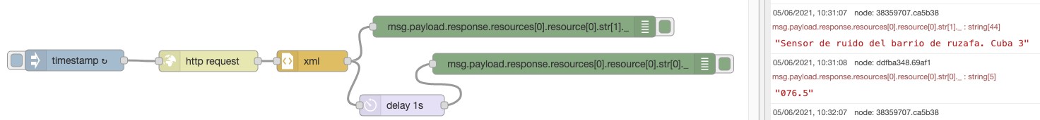
With only 6 nodes (included by default in the basic installation of Node-RED) we can build this flow or program that requests the data from the sensor installed in "Noise sensor in the Ruzafa neighbourhood. Cádiz 3" and return the noise value that is automatically updated every minute. You can see a demonstration video here.
Node-Red has many more possibilities, it is possible to combine several flows to make much more complex programmes or to build very visual dashboards like this one for final applications.
In short, in this article we have shown you how you don't need to know how to program or use complex software to make your own applications accessing open data in real time. You can get much more information on how to start using Node-RED here. You can also try other tools similar to Node-RED such as Apache Nify or ThingsBoard. We're sure the possibilities you can think of are endless - get creative!
[1] Equivalent continuous sound level. It is defined in ISO 1996-2:2017 as the value of the pressure level in dBA in A-weighting of a stable sound which in a time interval T has the same root mean square sound pressure as the sound being measured and whose level varies with time. In this case the period set for this sensor is 1 minute.
Content elaborated by Alejandro Alija, expert in Digital Transformation and Innovation.
Contents and points of view expressed in this publication are the exclusive responsibility of its author.
Blog
The visual representation of data helps our brain to digest large amounts of information quickly and easily. Interactive visualizations make it easier for non-experts to analyze complex situations represented as data.
As we introduced in our last post on this topic, graphical data visualization is a whole discipline within the universe of data science. In this new post we want to put the focus on interactive data visualizations. Dynamic visualizations allow the user to interact with data and transform it into graphs, tables and indicators that have the ability to display different information according to the filters set by the user. To a certain extent, interactive visualizations are an evolution of classic visualizations, allowing us to condense much more information in a space similar to the usual reports and presentations.
The evolution of digital technologies has shifted the focus of visual data analytics to the web and mobile environments. The tools and libraries that allow the generation and conversion of classic or static visualizations into dynamic or interactive ones are countless. However, despite the new formats of representation and generation of visualizations, sometimes there is a risk of forgetting the good practices of design and composition, which must always be present. The ease to condense large amounts of information into interactive visualisations can means that, on many occasions, users try to include a lot of information in a single graph and make even the simplest of reports unreadable. But, let's go back to the positive side of interactive visualizations and analyse some of their most significant advantages.
Benefits of interactive displays
The benefits of interactive data displays are several:
- Web and mobile technologies mainly. Interactive visualizations are designed to be consumed from modern software applications, many of them 100% web and mobile oriented. This makes them easy to read from any device.
- More information in the same space. The interactive displays show different information depending on the filters applied by the user. Thus, if we want to show the monthly evolution of the sales of a company according to the geography, in a classic visualization, we would use a bar chart (months in the horizontal axis and sales in the vertical axis) for each geography. On the contrary, in an interactive visualization, we use a single bar chart with a filter next to it, where we select the geography we want to visualize at each moment.
- Customizations. With interactive visualizations, the same report or dashboard can be customized for each user or groups of users. In this way, using filters as a menu, we can select some data or others, depending on the type and level of the user-consumer.
- Self-service. There are very simple interactive visualization technologies, which allow users to configure their own graphics and panels on demand by simply having the source data accessible. In this way, a non-expert user in visualization, can configure his own report with only dragging and dropping the fields he wants to represent.
Practical example
To illustrate with a practical example the above reasoning we will select a data se available in datos.gob.es data catalogue. In particular, we have chosen the air quality data of the Madrid City Council for the year 2020. This dataset contains the measurements (hourly granularity) of pollutants collected by the air quality network of the City of Madrid. In this dataset, we have the hourly time series for each pollutant in each measurement station of the Madrid City Council, from January to May 2020. For the interpretation of the dataset, it is also necessary to obtain the interpretation file in pdf format. Both files can be downloaded from the following website (It is also available through datos.gob.es).
Interactive data visualization tools
Thanks to the use of modern data visualization tools (in this case Microsoft Power BI, a free and easily accessible tool) we have been able to download the air quality data for 2020 (approximately half a million records) in just 30 minutes and create an interactive report. In this report, the end user can choose the measuring station, either by using the filter on the left or by selecting the station on the map below. In addition, the user can choose the pollutant he/she is interested in and a range of dates. In this static capture of the report, we have represented all the stations and all the pollutants. The objective is to see the significant reduction of pollution in all pollutants (except ozone due to the suppression of nitrogen oxides) due to the situation of sudden confinement caused by the Covid-19 pandemic since mid-March. To carry out this exercise we could have used other tools such as MS Excel, Qlik, Tableau or interactive visualization packages on programming environments such as R or Python. These tools are perfect for communicating data without the need for programming or coding skills.
In conclusion, the discipline of data visualization (Visual Analytics) is a huge field that is becoming very relevant today thanks to the proliferation of web and mobile interfaces wherever we look. Interactive visualizations empower the end user and democratize access to data analysis with codeless tools, improving transparency and rigor in communication in any aspect of life and society, such as science, politics and education.
Content elaborated by Alejandro Alija, expert in Digital Transformation and Innovation.
Contents and points of view expressed in this publication are the exclusive responsibility of its author.