How do I know if my prediction model is really good?

A few weeks ago, we told you about the different types of machine learning through a series of examples, and we analysed how to choose one or the other based on our objectives and the datasets available to train the algorithm.

Now let's assume that we have an already labelled dataset and we need to train a supervised learning model to solve the task at hand. At this point, we need some mechanism to tell us whether the model has learned correctly or not. That is what we are going to discuss in this post, the most used metrics to evaluate the quality of our models.

Model evaluation is a very important step in the development methodology of machine learning systems. It helps to measure the performance of the model, that is, to quantify the quality of the predictions it offers. To do this, we use evaluation metrics, which depend on the learning task we apply. As we saw in the previous post, within supervised learning there are two types of tasks that differ, mainly, in the type of output they offer:

• Classification tasks, which produce as output a discrete label, i.e. when the output is one within a finite set.
• Regression tasks, which output a continuous real value.

Here are some of the most commonly used metrics to assess the performance of both types of tasks:

Evaluation of classification models

In order to better understand these metrics, we will use as an example the predictions of a classification model to detect COVID patients. In the following table we can see in the first column the example identifier, in the second column the class predicted by the model, in the third column the actual class and the fourth column indicates whether the model has failed in its prediction or not. In this case, the positive class is "Yes" and the negative class is "No".

Examples of evaluation metrics for classification model include the following:

• Confusion matrix: this is a widely used tool that allows us to visually inspect and evaluate the predictions of our model. Each row represents the number of predictions of each class and the columns represent the instances of the actual class.

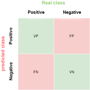
The description of each element of the matrix is as follows:

True Positive (VP): number of positive examples that the model predicts as positive. In the example above, VP is 1 (from example 6).

False positive (FP): number of negative examples that the model predicts as positive. In our example, FP is equal to 1 (from example 4).

False negative (FN): number of positive examples that the model predicts as negative. FN in the example would be 0.

True negative (VN): number of negative examples that the model predicts as negative. In the example, VN is 8.

• Accuracy: the fraction of predictions that the model made correctly.  It is represented as a percentage or a value between 0 and 1. It is a good metric when we have a balanced dataset, that is, when the number of labels of each class is similar. The accuracy of our example model is 0.9, since it got 9 predictions out of 10 correct. If our model had always predicted the "No" label, the accuracy would be 0.9 as well, but it does not solve our problem of identifying COVID patients.
• Recall: indicates the proportion of positive examples that are correctly identified by the model out of all actual positives. That is, VP / (VP + FN). In our example, the sensitivity value would be 1 / (1 + 0) = 1. If we were to evaluate with this metric, a model that always predicts the positive label ("Yes") would have a sensitivity of 1, but it would not be a very intelligent model. Although the ideal for our COVID detection model is to maximise sensitivity, this metric alone does not ensure that we have a good model.
• Precision: this metric is determined by the fraction of items correctly classified as positive among all items that the model has classified as positive. The formula is VP / (VP + FP). The example model would have an accuracy of 1 / (1 + 1) = 0.5. Let us now return to the model that always predicts the positive label. In that case, the accuracy of the model is 1 / (1 + 9) = 0.1. We see how this model had a maximum sensitivity, but has a very poor accuracy. In this case we need both metrics to evaluate the real quality of the model.
• F1 score: combines the Precision and Recall metrics to give a single score. This metric is the most appropriate when we have unbalanced datasets. It is calculated as the harmonic mean of Precision and Recall. The formula is F1 = (2 * precision * recall) / (precision + recall). You may wonder why we use the harmonic mean and not the simple mean. This is because the harmonic mean means that if one of the two measurements is small (even if the other is maximum), the value of F1 score is going to be small.

Evaluation of regression models

Unlike classification models, in regression models it is almost impossible to predict the exact value, but rather to be as close as possible to the real value, so most metrics, with subtle differences between them, are going to focus on measuring that: how close (or far) the predictions are from the real values.

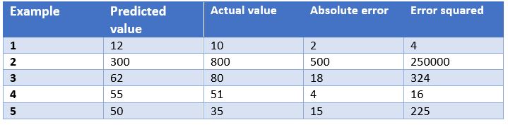
In this case, we have as an example the predictions of a model that determines the price of watches depending on their characteristics. In the table we show the price predicted by the model, the actual price, the absolute error and the squared error.

Some of the most common evaluation metrics for regression models are:

• Mean Absolute Error: This is the mean of the absolute differences between the target and predicted values. Since it is not squared, it does not penalise large errors, which makes it not very sensitive to outliers, so it is not a recommended metric in models where attention must be paid to outliers. This metric also represents the error on the same scale as the actual values. Ideally, its value should be close to zero. For our watch pricing model, the mean absolute error is 107.8.
• Mean Squared Errors: One of the most commonly used measures in regression work. It is simply the mean of the differences between the target and the predicted value squared. By squaring the errors, it magnifies large errors, so use it with care when we have outliers in our data set. It can take values between 0 and infinity. The closer the metric is to zero, the better. The mean square error of the example model is 50113.8. We see how in the case of our example large errors are magnified.
• Root Mean Squared Srror: This is equal to the square root of the previous metric. The advantage of this metric is that it presents the error in the same units as the target variable, which makes it easier to understand. For our model this error is equal to 223.86.
• R-squared: also called the coefficient of determination. This metric differs from the previous ones, as it compares our model with a basic model that always returns as prediction the mean of the training target values. The comparison between these two models is made on the basis of the mean squared errors of each model. The values this metric can take range from minus infinity to 1. The closer the value of this metric is to 1, the better our model is. The R-squared value for the model will be 0.455.
• Adjusted R-squared. An improvement of R-squared. The problem with the previous metric is that every time more independent variables (or predictor variables) are added to the model, R-squared stays the same or improves, but never gets worse, which can be confusing, because just because one model uses more predictor variables than another, it does not mean that it is better. Adjusted R-squared compensates for the addition of independent variables. The adjusted R-squared value will always be less than or equal to the R-squared value, but this metric will show improvement when the model is actually better. For this measure we cannot do the calculation for our example model because, as we have seen before, it depends on the number of examples and the number of variables used to train such a model.

Conclusion

When working with supervised learning algorithms it is very important to choose a correct evaluation metric for our model. For classification models it is very important to pay attention to the dataset and check whether it is balanced or not. For regression models we have to consider outliers and whether we want to penalise large errors or not.

Generally, however, the business domain will guide us in the right choice of metric. For a disease detection model, such as the one we have seen, we are interested in high sensitivity, but we are also interested in a good accuracy value, so F1-score would be a smart choice. On the other hand, in a model to predict the demand for a product (and therefore production), where overstocking may incur a storage cost overrun, it may be a good idea to use the mean squared errors to penalise large errors.

Content elaborated by Jose Antonio Sanchez, expert in Data Science and enthusiast of the Artificial Intelligence.

Contents and points of view expressed in this publication are the exclusive responsibility of its author.