28 data exercises found

Science and technology
Introduction
In previous content, we have explored in depth the exciting world of Large Language Models (LLM) and, in particular, the Retrieval Augmented Generation (RAG) techniques that are revolutionising the way we interact with conversational agents. This exercise marks a milestone in our series, as we will not only explain the concepts, but also guide you step-by-step in building your own RAG-powered conversational agent. For this, we will use a Google Colabnotebook.
Access the data lab repository on Github
Execute the data pre-processing code on Google Colab
Through this notebook, we will build a chat that uses RAG to improve its responses, starting from scratch. The notebook will guide the user through the whole process:
Installation of dependencies.
Setting up the environment.
Integration of a source of information in the form of a post.
Incorporation of this source into the chat knowledge base using RAG techniques.
Finally, we can see how the model's response changes before and after providing the post and asking a specific question about its content.
Tools used
Before starting, it is necessary to introduce and explain which tools we have used and why we have chosen them. For the construction of this RAG application we have used 3 pieces of technology or tools: Google Colab, OpenAI y LangChain. Both Google Colab and OpenAI are old acquaintances and we have used them several times in previous content. Therefore, in this section, we pay special attention to explaining what LangChain is, as it is a new tool that we have not used in previous posts.
Google Colab. As usual in our exercises, when computing resources are needed, as well as a user-friendly programming environment, we use Google Colab, as far as possible. Google Colab guarantees that any user who wants to reproduce the exercise can do so without complications derived from the configuration of the particular environments of each programmer. It should be noted that adapting this exercise inspired by previous resources available in LangChain to the Google Colab environment has been a challenge.
OpenAI. As a provider of the Chat GPT large language model (LLM), OpenAI offers a variety of powerful language models, such as GPT-4, GPT-4o, GPT-4o mini, etc. that are used to process and generate natural language text. In this case, the OpenAI language model is used in the answer generation area, where the user's question and the retrieved documents are combined to produce an accurate answer.
LangChain. It is an open source framework (set of libraries) designed to facilitate the development of large-scale language model (LLM) based applications. This framework is especially useful for integrating and managing complex flows that combine multiple components, such as language models, vector databases, and information retrieval tools, among others.
LangChain is widely used in the development of applications such as:
Question and answer systems (QA systems).
Virtual assistants with specific knowledge.
Customised text generation systems.
Data analysis tools based on natural language.
Key features of LangChain
Modularity and flexibility. LangChain is designed with a modular architecture that allows developers to connect different tools and services. This includes language models (such as OpenAI, Hugging Face, or local LLM) and vector databases (such as Pinecone, ChromaDB or Weaviate). The List of chat models that can be interacted with through Langchain is extensive.
Support for AGR (Generation Augmented Retrieval) techniques. Langhain facilitates the implementation of RAG techniques by enabling the direct integration of information retrieval and text generation models. This improves the accuracy of responses by enabling LLMs to work with up-to-date and specific knowledge.
Optimising the handling of prompts. Langhain helps to design and manage complex prompts efficiently. It allows to dynamically build a relevant context that works with the model, optimising the use of tokens and ensuring that responses are accurate and useful.
Tokens represent the basic units that an AI model uses to process text. A token can be a whole word, a part of a word or a punctuation mark. In the sentence "Hello world!" there are, for example, four different tokens: "Hello", "Hello", "World", "! Text processing requires more computational resources as the number of tokens increases. Free versions of AI models, including the one we use in this exercise, set limits on the number of tokens that can be processed.
Integrate multiple data sources. The framework can connect to various data sources, such as databases, APIs or user uploaded documents. This makes it ideal for building applications that need access to large volumes of structured or unstructured information.
Interoperability with multiple LLMs. LangChain is agnostic (can be adapted to various language model providers) with respect to the language model provider, which means that you can use OpenAI, Cohere, Anthropic or even locally hosted language models.
To conclude this section, it is worth noting the open source nature of Langhain, which facilitates collaboration and innovation in the development of applications based on language models. In addition, LangChain gives us incredible flexibility because it allows developers to easily integrate different LLMs, vectorisers and even final web interfaces into their applications.
Step-by-step exploration of the exercise: introduction to the Repository
The Github repository that we will use contains all the resources needed to build our RAG application. Inside, you will find:
README: this file provides an overview of the project, instructions for use and additional resources.
Jupyter Notebook: the example has been developed using a Jupyter Notebook format that we have already used in the past to code practical exercises combining a text document with code snippets executable in Google Colab. Here is the detailed implementation of the application, including data loading and processing, integration with language models such as GPT-44, configuration of information retrieval systems and generation of responses based on the retrieved data.
Notebook: preparing the Environment
Before starting, it is advisable to have the following requirements.
Basic knowledge of Python and Natural Language Processing (NLP): although the notebook is self-explanatory, a basic understanding of these concepts will facilitate learning.
Access to Google Colab: the notebook runs in this environment, which provides the necessary infrastructure.
Accounts active in OpenAI and LangChain with valid API keys. These services are free and essential for running the notebook. Once you register with these services, you will need to generate an API Key to interact with the services. You will need to have this key handy so that you can paste it when executing the corresponding code snippet. If you need help to get these keys, any conversational assistant such as chatGPT or Google Gemini can help you step-by-step to get the keys. If you need visual guidance on youtube you will find thousands of tutorials.
OpenAI API: https://openai.com/api/
Lanchain API: https://www.langchain.com/
Exploring the Notebook: block by block
The notebook is divided into several blocks, each dedicated to a specific stage of the development of our RAG application. In the following, we will describe each block in detail, including the code used and its explanation.
Note to user. In the following, we are going to reproduce blocks of the code present in the Colab notebook. For clarity we have divided the code into self-contained units and formatted the code to highlight the syntax of the Python programming language. In addition, the outputs provided by the Notebook have been formatted and highlighted in JSON format to make them more readable. Note that this Notebook invokes language model APIs and therefore the model response changes with each run. This means that the outputs (the answers) presented in this post may not be exactly the same as what the user receives when running the Notebook in Colab.
Block 1: Installation and initial configuration
import osos.kill(os.getpid(), 9)
It is very important that you run these two lines at the beginning of the exercise and then do not run it again until you close and exit Google Colab.
%%capture!pip install openai==1.55.3 httpx==0.27.2 --force-reinstall --quiet
!pip install langchain --quiet%pip install --quiet --upgrade langchain-text-splitters langchain-community
import getpassimport osos.environ["LANGCHAIN_TRACING_V2"] = "true"os.environ["LANGCHAIN_API_KEY"] = getpass.getpass()
When you run this snippet, a small dialogue box will appear below the snippet. There you must paste your Langchain API Key.
!pip install -qU langchain-openai!pip install -qU langgraph
import getpassimport osos.environ["OPENAI_API_KEY"] = getpass.getpass()from langchain_openai import ChatOpenAIllm = ChatOpenAI(model="gpt-4o-mini")
When you run this snippet, a small dialogue box will appear below the snippet. There you must paste your OpenAI API Key.
In this first block, we have installed the necessary libraries for our project. Some of the most relevant are:
openai: To interact with the OpenAI API and access models such as GPT-4.
langchain: A framework that simplifies LLM application development.
langchain-text-splitters: To break up long texts into smaller fragments that can be processed by language models.
langchain-community: A collection of additional tools and components for LangChain.
langchain-openai: To integrate LangChain with the OpenAI API.
langgraph: To visualise the workflow of our RAG application.
In addition to installing the libraries, we also set up the API keys for OpenAI and LangChain, using the getpass.getpass() function to enter them securely.
Block 2: Initialising the interaction with the LLM
Next, we start the first programmatic interaction (we pass our first prompt) with the language model. To check that everything works, we ask you to translate a simple sentence.
import getpass
import osos.environ["OPENAI_API_KEY"] = getpass.getpass()from langchain_openai import ChatOpenAIllm = ChatOpenAI(model="gpt-4o-mini")from langchain_core.messages import HumanMessage, SystemMessagemessages = [SystemMessage("Translate the following from English into Italian"),HumanMessage("hi!"),]llm.invoke(messages)
If everything went well we will get an output like this:
{ "content": "Ciao!", "additional_kwargs": { "refusal": null }, "response_metadata": { "token_usage": { "completion_tokens": 3, "prompt_tokens": 20, "total_tokens": 23, "completion_tokens_details": { "accepted_prediction_tokens": 0, "audio_tokens": 0, "reasoning_tokens": 0, "rejected_prediction_tokens": 0 }, "prompt_tokens_details": { "audio_tokens": 0, "cached_tokens": 0 } }, "model_name": "gpt-4o-mini-2024-07-18", "system_fingerprint": "fp_bd83329f63", "finish_reason": "stop", "logprobs": null }, "id": "run-ca631c07-fb63-47b2-8e78-339460c8a508-0", "usage_metadata": { "input_tokens": 20, "output_tokens": 3, "total_tokens": 23, "input_token_details": { "audio": 0, "cache_read": 0 }, "output_token_details": { "audio": 0, "reasoning": 0 } }}
This block is a basic introduction to using an LLM for a simple task: translation. The OpenAI API key is configured and a gpt-4o-mini language model is instantiated using ChatOpenAI.
Two messages are defined:
SystemMessage: Instruction to the model for translating from English into Italian.
HumanMessage: The text to be translated ("hi!").
Finally, the model is invoked with llm.invoke(messages) to get the translation.
Block 3: Creating Embeddings
To understand the concept of Embeddings applied to the context of natural language processing, we recommend reading this post.
import getpassos.environ["OPENAI_API_KEY"] = getpass.getpass()from langchain_openai import OpenAIEmbeddingsembeddings = OpenAIEmbeddings(model="text-embedding-3-large")
pip install -qU langchain-core
from langchain_core.vectorstores import InMemoryVectorStorevector_store = InMemoryVectorStore(embeddings)
When you run this snippet, a small dialogue box will appear below the snippet. There you must paste your OpenAI API Key.
This block focuses on the creation of embeddings (vector representations of text) that capture their semantic meaning. We use the OpenAIEmbeddings class to access OpenAI's text-embedding-3-large model, which generates high-quality embeddings .
The embeddings will be stored in an InMemoryVectorStore, an in-memory data structure that allows efficient searches based on semantic similarity.
Block 4: Implementing RAG
#RAGimport bs4from langchain_community.document_loaders import WebBaseLoader# Manten únicamente el título del post, los encabezados y el contenido del HTML bs4_strainer = bs4.SoupStrainer(class_=("post-title", "post-header", "post-content"))loader = WebBaseLoader(web_paths=("https://datos.gob.es/es/blog/slm-llm-rag-y-fine-tuning-pilares-de-la-ia…",))docs = loader.load()assert len(docs) == 1print(f"Total characters: {len(docs.page_content)}")from langchain_text_splitters import RecursiveCharacterTextSplittertext_splitter = RecursiveCharacterTextSplitter(chunk_size=1000,chunk_overlap=200,add_start_index=True,)all_splits = text_splitter.split_documents(docs)print(f"Split blog post into {len(all_splits)} sub-documents.")document_ids = vector_store.add_documents(documents=all_splits)print(document_ids[:3])
This block is the heart of the RAG implementation. Start loading the content of a post, using WebBaseLoader and the URL of the post on SLM, LLM, RAG and Fine-tuning..
To prepare our Generation Augmented Retrieval (GAR) system, we start by processing the text of the post using segmentation techniques. This initial step is crucial, as we break down the content into smaller fragments that are complete in meaning. We use LangChain tools to perform this segmentation, assigning each fragment a unique identifier (id). This prior preparation allows us to subsequently perform efficient and accurate searches when the system needs to retrieve relevant information to answer queries.
The bs4.SoupStrainer is used to extract only the relevant sections of the HTML. The text of the post is split into smaller fragments with RecursiveCharacterTextSplitter, ensuring overlap between fragments to maintain context. These fragments are added to the vector_store created in the previous block, generating embeddings for each one.
We see that the result of one of the fragments informs us that it has split the document into 21 sub-documents.
Split blog post into 21 sub-documents.
Documents have their own identifier. For example, the first 3 are identified as:.
["409f1bcb-1710-49b0-80f8-e45b7ca51a96", "e242f16c-71fd-4e7b-8b28-ece6b1e37a1c", "9478b11c-61ab-4dac-9903-f8485c4770c6"]
Block 5: Defining the Prompt and visualising the workflow
from langchain import hubprompt = hub.pull("rlm/rag-prompt")example_messages = prompt.invoke({"context": "(context goes here)", "question": "(question goes here)"}).to_messages()assert len(example_messages) == 1print(example_messages.content)from langchain_core.documents import Documentfrom typing_extensions import List, TypedDictclass State(TypedDict):question: strcontext: List[Document]answer: strdef retrieve(state: State):retrieved_docs = vector_store.similarity_search(state["question"])return {"context": retrieved_docs}def generate(state: State):docs_content = "\n\n".join(doc.page_content for doc in state["context"])messages = prompt.invoke({"question": state["question"], "context": docs_content})response = llm.invoke(messages)return {"answer": response.content}from langgraph.graph import START, StateGraphgraph_builder = StateGraph(State).add_sequence([retrieve, generate])graph_builder.add_edge(START, "retrieve")graph = graph_builder.compile()from IPython.display import Image, displaydisplay(Image(graph.get_graph().draw_mermaid_png()))result = graph.invoke({"question": "What is Task Decomposition?"})print(f"Context: {result["context"]}\n\n")print(f"Answer: {result["answer"]}")for step in graph.stream({"question": "¿Cual es el futuro de la IA Generativa?"}, stream_mode="updates"):print(f"{step}\n\n----------------\n")
This block defines the prompt to be used to interact with the LLM. A predefined LangChain Hub prompt (rlm/rag-prompt) is used which is designed for RAG tasks.
Two functions are defined:
retrieve: search the vector_store for snippets most similar to the user's question.
generate: generates a response using the LLM, taking into account the context provided by the retrieved fragments.
langgraph is used to visualise the RAG workflow.
Figure 1: RAG workflow. Own elaboration.
Finally, the system is tested with two questions: one in English ("What is Task Decomposition?") and one in Spanish ("¿Cual es el futuro de la AI Generativa?").
The first question, "What is Task Decomposition?", is in English and is a generic question, unrelated to our content post. Therefore, although the system searches in its knowledge base previously created with the vectorisation of the document (post), it does not find any relation between the question and this context.
This text may vary with each execution
Answer: There is no explicit mention of the concept of "Task Decomposition" in the context provided. Therefore, I have no information on what Task Decomposition is.
Answer: Task Decomposition is a process that decomposes a complex task into smaller, more manageable sub-tasks. This allows each subtask to be addressed independently, facilitating their resolution and improving overall efficiency. Although the context provided does not explicitly define Task Decomposition, this concept is common in AI and task optimisation.
Answer: Task Decomposition is a process that decomposes a complex task into smaller, more manageable sub-tasks. This allows each subtask to be addressed independently, facilitating their resolution and improving overall efficiency. Although the context provided does not explicitly define Task Decomposition, this concept is common in AI and task optimisation.
{ "retrieve": { "context": [ { "id": "53962c40-c08b-4547-a74a-26f63cced7e8", "metadata": { "source": "https://datos.gob.es/es/blog/slm-llm-rag-y-fine-tuning-pilares-de-la-ia…", "title": "SLM, LLM, RAG y Fine-tuning: Pilares de la IA Generativa Moderna | datos.gob.es", "description": "En el vertiginoso mundo de la Inteligencia Artificial (IA) Generativa, encontramos diversos conceptos que se han convertido en fundamentales para comprender y aprovechar el potencial de esta tecnología. Hoy nos centramos en cuatro: los Modelos de Lenguaje Pequeños (SLM, por sus siglas en inglés), los Modelos de Lenguaje Grandes (LLM), la Generación Aumentada por Recuperación", "language": "es", "start_index": 12763 }, "page_content": "La verdadera magia ocurre cuando estos elementos se combinan de formas innovadoras, creando sistemas de IA Generativa más potentes, precisos y adaptables que nunca. A medida que estas tecnologías continúen evolucionando, podemos esperar ver aplicaciones cada vez más sofisticadas y útiles en una amplia gama de campos, desde la atención médica hasta la creación de contenido creativo.\nEl desafío para los desarrolladores e investigadores será encontrar el equilibrio óptimo entre estos elementos, considerando factores como la eficiencia computacional, la precisión, la adaptabilidad y la ética. El futuro de la IA Generativa promete ser fascinante, y estos cuatro conceptos estarán sin duda en el centro de su desarrollo y aplicación en los años venideros." }, { "id": "2dcdfcb3-e9cf-440b-a08a-6db6d5ddb356", "metadata": { "source": "https://datos.gob.es/es/blog/slm-llm-rag-y-fine-tuning-pilares-de-la-ia…", "title": "SLM, LLM, RAG y Fine-tuning: Pilares de la IA Generativa Moderna | datos.gob.es", "description": "En el vertiginoso mundo de la Inteligencia Artificial (IA) Generativa, encontramos diversos conceptos que se han convertido en fundamentales para comprender y aprovechar el potencial de esta tecnología. Hoy nos centramos en cuatro: los Modelos de Lenguaje Pequeños (SLM, por sus siglas en inglés), los Modelos de Lenguaje Grandes (LLM), la Generación Aumentada por Recuperación", "language": "es", "start_index": 11496 }, "page_content": "Conclusiones y futuro de la IA\nLa combinación de estos cuatro pilares está abriendo nuevas posibilidades en el campo de la IA Generativa:\n\nSistemas híbridos: combinación de SLM y LLM para diferentes aspectos de una misma aplicación, optimizando rendimiento y eficiencia.\nRAG avanzado: implementación de sistemas RAG más sofisticados que utilicen múltiples fuentes de información y técnicas de recuperación más avanzadas.\nFine-tuning continuo: desarrollo de técnicas para el ajuste continuo de modelos en tiempo real, adaptándose a nuevos datos y necesidades.\nPersonalización a escala: creación de modelos altamente personalizados para individuos o pequeños grupos, combinando fine-tuning y RAG.\nIA Generativa ética y responsable: implementación de estas técnicas con un enfoque en la transparencia, la verificabilidad y la reducción de sesgos." }, { "id": "9478b11c-61ab-4dac-9903-f8485c4770c6", "metadata": { "source": "https://datos.gob.es/es/blog/slm-llm-rag-y-fine-tuning-pilares-de-la-ia…", "title": "SLM, LLM, RAG y Fine-tuning: Pilares de la IA Generativa Moderna | datos.gob.es", "description": "En el vertiginoso mundo de la Inteligencia Artificial (IA) Generativa, encontramos diversos conceptos que se han convertido en fundamentales para comprender y aprovechar el potencial de esta tecnología. Hoy nos centramos en cuatro: los Modelos de Lenguaje Pequeños (SLM, por sus siglas en inglés), los Modelos de Lenguaje Grandes (LLM), la Generación Aumentada por Recuperación", "language": "es", "start_index": 1341 }, "page_content": "Fecha de la noticia: 09-09-2024\n\nEn el vertiginoso mundo de la Inteligencia Artificial (IA) Generativa, encontramos diversos conceptos que se han convertido en fundamentales para comprender y aprovechar el potencial de esta tecnología. Hoy nos centramos en cuatro: los Modelos de Lenguaje Pequeños (SLM, por sus siglas en inglés), los Modelos de Lenguaje Grandes (LLM), la Generación Aumentada por Recuperación (RAG) y el Fine-tuning. En este artículo, exploraremos cada uno de estos términos, sus interrelaciones y cómo están moldeando el futuro de la IA generativa.\nEmpecemos por el principio. Definiciones." }, { "id": "d6dd28f3-5a20-4cee-8cbf-6bc39adbf098", "metadata": { "source": "https://datos.gob.es/es/blog/slm-llm-rag-y-fine-tuning-pilares-de-la-ia…", "title": "SLM, LLM, RAG y Fine-tuning: Pilares de la IA Generativa Moderna | datos.gob.es", "description": "En el vertiginoso mundo de la Inteligencia Artificial (IA) Generativa, encontramos diversos conceptos que se han convertido en fundamentales para comprender y aprovechar el potencial de esta tecnología. Hoy nos centramos en cuatro: los Modelos de Lenguaje Pequeños (SLM, por sus siglas en inglés), los Modelos de Lenguaje Grandes (LLM), la Generación Aumentada por Recuperación", "language": "es", "start_index": 12341 }, "page_content": "SLM, LLM, RAG y Fine-tuning representan los pilares fundamentales sobre los que se está construyendo el futuro de la IA Generativa. Cada uno de estos conceptos aporta fortalezas únicas:\n\nLos SLM ofrecen eficiencia y especialización.\nLos LLM proporcionan versatilidad y capacidad de generalización.\nRAG mejora la precisión y relevancia de las respuestas.\nEl Fine-tuning permite la adaptación y personalización de modelos." } ] }}
As you can see in the response, the system retrieves 4 documents (in the diagram above, this corresponds to the "Retrieve" stage) with their corresponding "id" (identifiers), for example, the first document "id":. "53962c40-c08b-4547-a74a-26f63cced7e8" which corresponds to a fragment of the original post "title":. "SLM, LLM, RAG and Fine-tuning: Pillars of Modern Generative AI | datos.gob.es".
With these 4 fragments the system considers that it has enough relevant information to provide (in the diagram above, the "generate" stage) a satisfactory answer to the question.
{ "generate": { "answer": "El futuro de la IA Generativa promete ser fascinante, con el desarrollo de sistemas más potentes, precisos y adaptables gracias a la combinación de los modelos de lenguaje pequeños (SLM), los grandes (LLM), la generación aumentada por recuperación (RAG) y el fine-tuning. Esperamos ver aplicaciones cada vez más sofisticadas en campos como la atención médica y la creación de contenido creativo, mientras se busca un equilibrio entre eficiencia, precisión y ética. La implementación de estas tecnologías con un enfoque ético y responsable será clave en su evolución." }}
Bloque 6: personalizando el prompt
from langchain_core.prompts import PromptTemplatetemplate = """Use the following pieces of context to answer the question at the end.If you don"t know the answer, just say that you don"t know, don"t try to make up an answer.Use three sentences maximum and keep the answer as concise as possible.Always say "thanks for asking!" at the end of the answer.{context}Question: {question}Helpful Answer:"""custom_rag_prompt = PromptTemplate.from_template(template)
This block customises the prompt to make answers more concise and add a polite sentence at the end. PromptTemplate is used to create a new prompt with the desired instructions.
Block 7: Adding metadata and refining your search
total_documents = len(all_splits)third = total_documents // 3for i, document in enumerate(all_splits):if i < third:document.metadata["section"] = "beginning"elif i < 2 * third:document.metadata["section"] = "middle"else:document.metadata["section"] = "end"all_splits.metadatafrom langchain_core.vectorstores import InMemoryVectorStorevector_store = InMemoryVectorStore(embeddings)_ = vector_store.add_documents(all_splits)from typing import Literalfrom typing_extensions import Annotatedclass Search(TypedDict):"""Search query."""query: Annotated[str, ..., "Search query to run."]section: Annotated(Literal["beginning", "middle", "end"],...,"Section to query.",]class State(TypedDict):question: strquery: Searchcontext: List[Document]answer: strdef analyze_query(state: State):structured_llm = llm.with_structured_output(Search)query = structured_llm.invoke(state["question"])return {"query": query}def retrieve(state: State):query = state["query"]retrieved_docs = vector_store.similarity_search(query["query"],filter=lambda doc: doc.metadata.get("section") == query["section"],)return {"context": retrieved_docs}def generate(state: State):docs_content = "\n\n".join(doc.page_content for doc in state["context"])messages = prompt.invoke({"question": state["question"], "context": docs_content})response = llm.invoke(messages)return {"answer": response.content}graph_builder = StateGraph(State).add_sequence([analyze_query, retrieve, generate])graph_builder.add_edge(START, "analyze_query")graph = graph_builder.compile()display(Image(graph.get_graph().draw_mermaid_png()))for step in graph.stream({"question": "¿Cual es el furturo de la IA Generativa en palabras del autor?"},stream_mode="updates",):print(f"{step}\n\n----------------\n")
In this block, metadata is added to the post fragments, dividing them into three sections: "beginning", "middle" and "end". This allows for more refined searches, limiting the search to a specific section of the post.
A new analyze_query function is introduced that uses the LLM to determine the section of the post most relevant to the user's question. The RAG workflow is updated to include this new step.
Finally, the system is tested with a question in Spanish ("What is the future of Generative AI in the author's words?"), observing how the system uses the information in the "end" section of the post to generate a more accurate answer.
Let's look at the result:
Figure 2: RAG workflow. Own elaboration.
{ "analyze_query": { "query": { "query": "futuro de la IA Generativa", "section": "end" } }}----------------{ "retrieve": { "context": [ { "id": "887fa76d-5bda-41fb-8976-eca46cff194e", "metadata": { "source": "https://datos.gob.es/es/blog/slm-llm-rag-y-fine-tuning-pilares-de-la-ia…", "title": "SLM, LLM, RAG y Fine-tuning: Pilares de la IA Generativa Moderna | datos.gob.es", "description": "En el vertiginoso mundo de la Inteligencia Artificial (IA) Generativa, encontramos diversos conceptos que se han convertido en fundamentales para comprender y aprovechar el potencial de esta tecnología. Hoy nos centramos en cuatro: los Modelos de Lenguaje Pequeños (SLM, por sus siglas en inglés), los Modelos de Lenguaje Grandes (LLM), la Generación Aumentada por Recuperación", "language": "es", "start_index": 11496, "section": "end" }, "page_content": "Conclusiones y futuro de la IA\nLa combinación de estos cuatro pilares está abriendo nuevas posibilidades en el campo de la IA Generativa: Sistemas híbridos: combinación de SLM y LLM para diferentes aspectos de una misma aplicación, optimizando rendimiento y eficiencia. RAG avanzado: implementación de sistemas RAG más sofisticados que utilicen múltiples fuentes de información y técnicas de recuperación más avanzadas. Fine-tuning continuo: desarrollo de técnicas para el ajuste continuo de modelos en tiempo real, adaptándose a nuevos datos y necesidades. Personalización a escala: creación de modelos altamente personalizados para individuos o pequeños grupos, combinando fine-tuning y RAG. IA Generativa ética y responsable: implementación de estas técnicas con un enfoque en la transparencia, la verificabilidad y la reducción de sesgos." }, { "id": "383ed352-8245-40e1-8249-7efbc6cbfd28", "metadata": { "source": "https://datos.gob.es/es/blog/slm-llm-rag-y-fine-tuning-pilares-de-la-ia…", "title": "SLM, LLM, RAG y Fine-tuning: Pilares de la IA Generativa Moderna | datos.gob.es", "description": "En el vertiginoso mundo de la Inteligencia Artificial (IA) Generativa, encontramos diversos conceptos que se han convertido en fundamentales para comprender y aprovechar el potencial de esta tecnología. Hoy nos centramos en cuatro: los Modelos de Lenguaje Pequeños (SLM, por sus siglas en inglés), los Modelos de Lenguaje Grandes (LLM), la Generación Aumentada por Recuperación", "language": "es", "start_index": 12763, "section": "end" }, "page_content": "La verdadera magia ocurre cuando estos elementos se combinan de formas innovadoras, creando sistemas de IA Generativa más potentes, precisos y adaptables que nunca. A medida que estas tecnologías continúen evolucionando, podemos esperar ver aplicaciones cada vez más sofisticadas y útiles en una amplia gama de campos, desde la atención médica hasta la creación de contenido creativo. El desafío para los desarrolladores e investigadores será encontrar el equilibrio óptimo entre estos elementos, considerando factores como la eficiencia computacional, la precisión, la adaptabilidad y la ética. El futuro de la IA Generativa promete ser fascinante, y estos cuatro conceptos estarán sin duda en el centro de su desarrollo y aplicación en los años venideros." }, { "id": "d0fd32fa-5fb9-49a1-9d23-7368cb3d30e2", "metadata": { "source": "https://datos.gob.es/es/blog/slm-llm-rag-y-fine-tuning-pilares-de-la-ia…", "title": "SLM, LLM, RAG y Fine-tuning: Pilares de la IA Generativa Moderna | datos.gob.es", "description": "En el vertiginoso mundo de la Inteligencia Artificial (IA) Generativa, encontramos diversos conceptos que se han convertido en fundamentales para comprender y aprovechar el potencial de esta tecnología. Hoy nos centramos en cuatro: los Modelos de Lenguaje Pequeños (SLM, por sus siglas en inglés), los Modelos de Lenguaje Grandes (LLM), la Generación Aumentada por Recuperación", "language": "es", "start_index": 12341, "section": "end" }, "page_content": "SLM, LLM, RAG y Fine-tuning representan los pilares fundamentales sobre los que se está construyendo el futuro de la IA Generativa. Cada uno de estos conceptos aporta fortalezas únicas: Los SLM ofrecen eficiencia y especialización. Los LLM proporcionan versatilidad y capacidad de generalización. RAG mejora la precisión y relevancia de las respuestas. El Fine-tuning permite la adaptación y personalización de modelos." }, { "id": "c064efe8-e782-4fde-9944-9a1ffd88ff7f", "metadata": { "source": "https://datos.gob.es/es/blog/slm-llm-rag-y-fine-tuning-pilares-de-la-ia…", "title": "SLM, LLM, RAG y Fine-tuning: Pilares de la IA Generativa Moderna | datos.gob.es", "description": "En el vertiginoso mundo de la Inteligencia Artificial (IA) Generativa, encontramos diversos conceptos que se han convertido en fundamentales para comprender y aprovechar el potencial de esta tecnología. Hoy nos centramos en cuatro: los Modelos de Lenguaje Pequeños (SLM, por sus siglas en inglés), los Modelos de Lenguaje Grandes (LLM), la Generación Aumentada por Recuperación", "language": "es", "start_index": 13522, "section": "end" }, "page_content": "Contenido elaborado por Alejandro Alija, experto en Transformación Digital e Innovación. Los contenidos y los puntos de vista reflejados en esta publicación son responsabilidad exclusiva de su autor. inteligencia artificial procesamiento del lenguaje natural PLN RAG LLM SLM fine-tuning algoritmos deep learning" } ] }}
{ "generate": { "answer": "El futuro de la IA Generativa se centra en la combinación de SLM, LLM, RAG y fine-tuning, que permiten crear sistemas más potentes, precisos y adaptables. A medida que estas tecnologías evolucionen, se espera ver aplicaciones sofisticadas en diversos campos. Sin embargo, el reto será equilibrar eficiencia, precisión, adaptabilidad y ética en su desarrollo." }}
Conclusions
Through this notebook tour of Google Colab, we have experienced first-hand the construction of a conversational agent with RAG. We have learned to:
Install the necessary libraries.
Configure the development environment.
Upload and process data.
Create embeddings and store them in a vector_store.
Implement the RAG recovery and generation stages.
Customise the prompt to get more specific answers.
Add metadata to refine the search.
This practical exercise provides you with the tools and knowledge you need to start exploring the potential of RAG and develop your own applications.
Dare to experiment with different information sources, language models and prompts to create increasingly sophisticated conversational agents!
Content prepared by Alejandro Alija, expert in Digital Transformation and Innovation. The contents and points of view reflected in this publication are the sole responsibility of its author.


Science and technology
Open data portals are an invaluable source of public information. However, extracting meaningful insights from this data can be challenging for users without advanced technical knowledge.
In this practical exercise, we will explore the development of a web application that democratizes access to this data through the use of artificial intelligence, allowing users to make queries in natural language.
The application, developed using the datos.gob.es portal as a data source, integrates modern technologies such as Streamlit for the user interface and Google's Gemini language model for natural language processing. The modular nature allows any Artificial Intelligence model to be used with minimal changes. The complete project is available in the Github repository.
Access the data laboratory repository on Github
Run the data preprocessing code Google Colab
In this video, the author explains what you will find both on Github and Google Colab.
Application Architecture
The core of the application is based on four main interconnected sections that work together to process user queries:
Context Generation
Analyzes the characteristics of the chosen dataset.
Generates a detailed description including dimensions, data types, and statistics.
Creates a structured template with specific guidelines for code generation.
Context and Query Combination
Combines the generated context with the user's question, creating the prompt that the artificial intelligence model will receive.
Response Generation
Sends the prompt to the model and obtains the Python code that allows solving the generated question.
Code Execution
Safely executes the generated code with a retry and automatic correction system.
Captures and displays the results in the application frontend.
Figure 1. Request processing flow
Development Process
The first step is to establish a way to access public data. The datos.gob.es portal offers datasets via API. Functions have been developed to navigate the catalog and download these files efficiently.
Figura 2. API de datos.gob
The second step addresses the question: how to convert natural language questions into useful data analysis? This is where Gemini, Google's language model, comes in. However, it's not enough to simply connect the model; it's necessary to teach it to understand the specific context of each dataset.
A three-layer system has been developed:
A function that analyzes the dataset and generates a detailed "technical sheet".
Another that combines this sheet with the user's question.
And a third that translates all this into executable Python code.
You can see in the image below how this process develops and, subsequently, the results of the generated code are shown once executed.
Figure 3. Visualization of the application's response processing
Finally, with Streamlit, a web interface has been built that shows the process and its results to the user. The interface is as simple as choosing a dataset and asking a question, but also powerful enough to display complex visualizations and allow data exploration.
The final result is an application that allows anyone, regardless of their technical knowledge, to perform data analysis and learn about the code executed by the model. For example, a municipal official can ask "What is the average age of the vehicle fleet?" and get a clear visualization of the age distribution.
Figure 4. Complete use case. Visualizing the distribution of registration years of the municipal vehicle fleet of Almendralejo in 2018
What Can You Learn?
This practical exercise allows you to learn:
AI Integration in Web Applications:
How to communicate effectively with language models like Gemini.
Techniques for structuring prompts that generate precise code.
Strategies for safely handling and executing AI-generated code.
Web Development with Streamlit:
Creating interactive interfaces in Python.
Managing state and sessions in web applications.
Implementing visual components for data.
Working with Open Data:
Connecting to and consuming public data APIs.
Processing Excel files and DataFrames.
Data visualization techniques.
Development Best Practices:
Modular structuring of Python code.
Error handling and retries.
Implementation of visual feedback systems.
Web application deployment using ngrok.
Conclusions and Future
This exercise demonstrates the extraordinary potential of artificial intelligence as a bridge between public data and end users. Through the practical case developed, we have been able to observe how the combination of advanced language models with intuitive interfaces allows us to democratize access to data analysis, transforming natural language queries into meaningful analysis and informative visualizations.
For those interested in expanding the system's capabilities, there are multiple promising directions for its evolution:
Incorporation of more advanced language models that allow for more sophisticated analysis.
Implementation of learning systems that improve responses based on user feedback.
Integration with more open data sources and diverse formats.
Development of predictive and prescriptive analysis capabilities.
In summary, this exercise not only demonstrates the feasibility of democratizing data analysis through artificial intelligence, but also points to a promising path toward a future where access to and analysis of public data is truly universal. The combination of modern technologies such as Streamlit, language models, and visualization techniques opens up a range of possibilities for organizations and citizens to make the most of the value of open data.

Science and technology
Open data portals play a fundamental role in accessing and reusing public information. A key aspect in these environments is the tagging of datasets, which facilitates their organization and retrieval.
Word embeddings represent a transformative technology in the field of natural language processing, allowing words to be represented as vectors in a multidimensional space where semantic relationships are mathematically preserved. This exercise explores their practical application in a tag recommendation system, using the datos.gob.es open data portal as a case study.
The exercise is developed in a notebook that integrates the environment configuration, data acquisition, and recommendation system processing, all implemented in Python. The complete project is available in the Github repository.
Access the data lab repository on GitHub
Run the data preprocessing code on Google Colab
In this video, the author explains what you will find both on Github and Google Colab (English subtitles available).
Understanding word embeddings
Word embeddings are numerical representations of words that revolutionize natural language processing by transforming text into a mathematically processable format. This technique encodes each word as a numerical vector in a multidimensional space, where the relative position between vectors reflects semantic and syntactic relationships between words. The true power of embeddings lies in three fundamental aspects:
Context capture: unlike traditional techniques such as one-hot encoding, embeddings learn from the context in which words appear, allowing them to capture meaning nuances.
Semantic algebra: the resulting vectors allow mathematical operations that preserve semantic relationships. For example, vector('Madrid') - vector('Spain') + vector('France') ≈ vector('Paris'), demonstrating the capture of capital-country relationships.
Quantifiable similarity: similarity between words can be measured through metrics, allowing identification of not only exact synonyms but also terms related in different degrees and generalizing these relationships to new word combinations.
In this exercise, pre-trained GloVe (Global Vectors for Word Representation) embeddings were used, a model developed by Stanford that stands out for its ability to capture global semantic relationships in text. In our case, we use 50-dimensional vectors, a balance between computational complexity and semantic richness. To comprehensively evaluate its ability to represent Spanish language, multiple tests were conducted:
Word similarity was analyzed using cosine similarity, a metric that evaluates the angle between two word vectors. This measure results in values between -1 and 1, where values close to 1 indicate high semantic similarity, while values close to 0 indicate little or no relationship. Terms like "amor" (love), "trabajo" (work), and "familia" (family) were evaluated to verify that the model correctly identified semantically related words.
The model's ability to solve linguistic analogies was tested, for example, "hombre es a mujer lo que rey es a reina" (Man is to woman what king is to queen), confirming its ability to capture complex semantic relationships.
Vector operations were performed (such as "rey - hombre + mujer") to check if the results maintained semantic coherence.
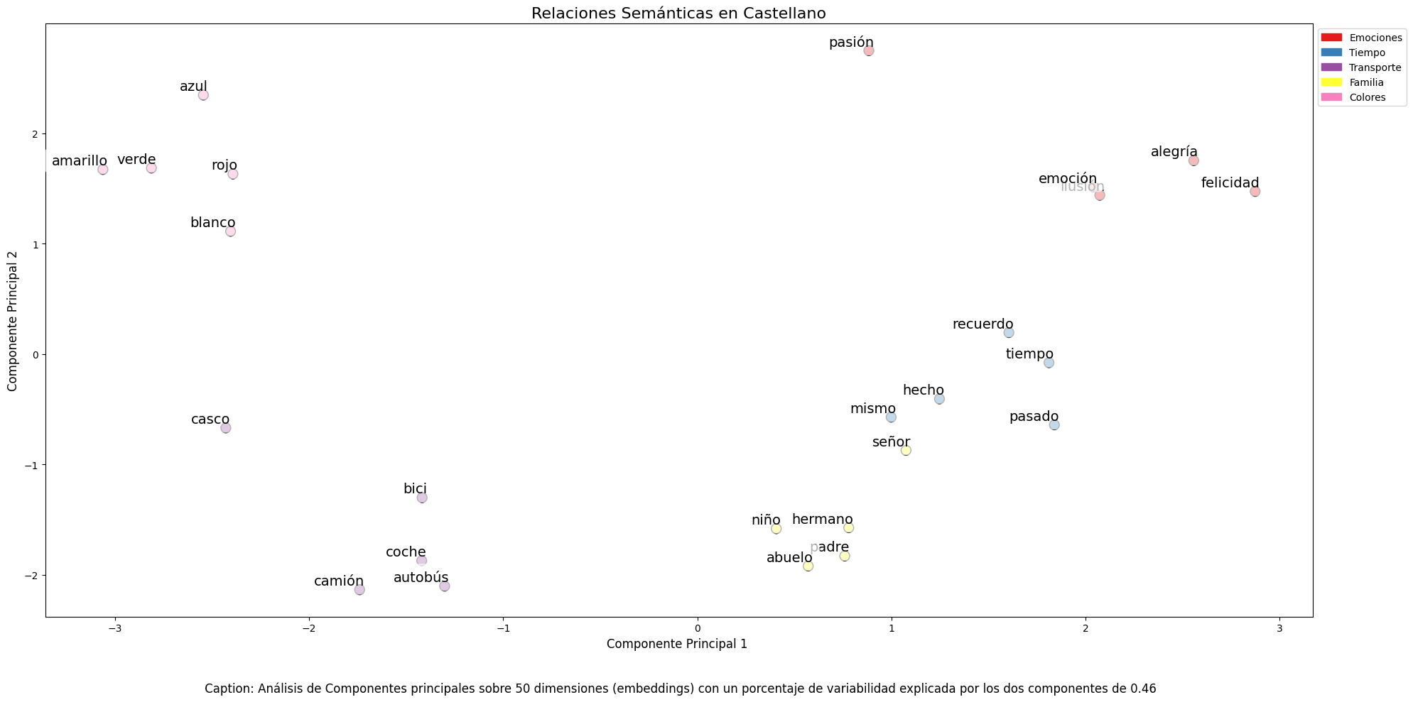
Finally, dimensionality reduction techniques were applied to a representative sample of 40 Spanish words, allowing visualization of semantic relationships in a two-dimensional space. The results revealed natural grouping patterns among semantically related terms, as observed in the figure:
Emotions: alegría (joy), felicidad (happiness) or pasión (passion) appear grouped in the upper right.
Family-related terms: padre (father), hermano (brother) or abuelo (grandfather) concentrate at the bottom.
Transport: coche (car), autobús (bus), or camión (truck) form a distinctive group.
Colors: azul (blue), verde (green) or rojo (red) appear close to each other.
Figure 1. Principal Components Analysis on 50 dimensions (embeddings) with an explained variability percentage by the two components of 0.46
To systematize this evaluation process, a unified function has been developed that encapsulates all the tests described above. This modular architecture allows automatic and reproducible evaluation of different pre-trained embedding models, thus facilitating objective comparison of their performance in Spanish language processing. The standardization of these tests not only optimizes the evaluation process but also establishes a consistent framework for future comparisons and validations of new models by the public.
The good capacity to capture semantic relationships in Spanish language is what we leverage in our tag recommendation system.
Embedding-based Recommendation System
Leveraging the properties of embeddings, we developed a tag recommendation system that follows a three-phase process:
Embedding generation: for each dataset in the portal, we generate a vector representation combining the title and description. This allows us to compare datasets by their semantic similarity.
Similar dataset identification: using cosine similarity between vectors, we identify the most semantically similar datasets.
Tag extraction and standardization: from similar sets, we extract their associated tags and map them with Eurovoc thesaurus terms. This thesaurus, developed by the European Union, is a multilingual controlled vocabulary that provides standardized terminology for cataloging documents and data in the field of European policies. Again, leveraging the power of embeddings, we identify the semantically closest Eurovoc terms to our tags, thus ensuring coherent standardization and better interoperability between European information systems.
The results show that the system can generate coherent and standardized tag recommendations. To illustrate the system's operation, let's take the case of the dataset "Tarragona City Activities Agenda":
Figure 2. Tarragona City Events Guide
The system:
Finds similar datasets like "Terrassa Activities Agenda" and "Barcelona Cultural Agenda".
Identifies common tags from these datasets, such as "EXHIBITIONS", "THEATER", and "CULTURE".
Suggests related Eurovoc terms: "cultural tourism", "cultural promotion", and "cultural industry".
Advantages of the Approach
This approach offers significant advantages:
Contextual Recommendations: the system suggests tags based on the real meaning of the content, not just textual matches.
Automatic Standardization: integration with Eurovoc ensures a controlled and coherent vocabulary.
Continuous Improvement: the system learns and improves its recommendations as new datasets are added.
Interoperability: the use of Eurovoc facilitates integration with other European systems.
Conclusions
This exercise demonstrates the great potential of embeddings as a tool for associating texts based on their semantic nature. Through the analyzed practical case, it has been possible to observe how, by identifying similar titles and descriptions between datasets, precise recommendations of tags or keywords can be generated. These tags, in turn, can be linked with keywords from a standardized thesaurus like Eurovoc, applying the same principle.
Despite the challenges that may arise, implementing these types of systems in production environments presents a valuable opportunity to improve information organization and retrieval. The accuracy in tag assignment can be influenced by various interrelated factors in the process:
The specificity of dataset titles and descriptions is fundamental, as correct identification of similar content and, therefore, adequate tag recommendation depends on it.
The quality and representativeness of existing tags in similar datasets directly determines the relevance of generated recommendations.
The thematic coverage of the Eurovoc thesaurus, which, although extensive, may not cover specific terms needed to describe certain datasets precisely.
The vectors' capacity to faithfully capture semantic relationships between content, which directly impacts the precision of assigned tags.
For those who wish to delve deeper into the topic, there are other interesting approaches to using embeddings that complement what we've seen in this exercise, such as:
Using more complex and computationally expensive embedding models (like BERT, GPT, etc.)
Training models on a custom domain-adapted corpus.
Applying deeper data cleaning techniques.
In summary, this exercise not only demonstrates the effectiveness of embeddings for tag recommendation but also unlocks new possibilities for readers to explore all the possibilities this powerful tool offers.
Tourism
Science and technology
1. Introduction
Visualizations are graphical representations of data that allow for the simple and effective communication of information linked to them. The possibilities for visualization are very broad, from basic representations such as line graphs, bar charts or relevant metrics, to visualizations configured on interactive dashboards.
In this section "Visualizations step by step" we are periodically presenting practical exercises using open data available on datos.gob.es or other similar catalogs. In them, the necessary steps to obtain the data, perform the transformations and relevant analyses to, finally obtain conclusions as a summary of said information, are addressed and described in a simple way.
Each practical exercise uses documented code developments and free-to-use tools. All generated material is available for reuse in the GitHub repository of datos.gob.es.
In this specific exercise, we will explore tourist flows at a national level, creating visualizations of tourists moving between autonomous communities (CCAA) and provinces.
Access the data laboratory repository on Github
Execute the data pre-processing code on Google Colab
In this video, the author explains what you will find on both Github and Google Colab.
2. Context
Analyzing national tourist flows allows us to observe certain well-known movements, such as, for example, that the province of Alicante is a very popular summer tourism destination. In addition, this analysis is interesting for observing trends in the economic impact that tourism may have, year after year, in certain CCAA or provinces. The article on experiences for the management of visitor flows in tourist destinations illustrates the impact of data in the sector.
3. Objective
The main objective of the exercise is to create interactive visualizations in Python that allow visualizing complex information in a comprehensive and attractive way. This objective will be met using an open dataset that contains information on national tourist flows, posing several questions about the data and answering them graphically. We will be able to answer questions such as those posed below:
In which CCAA is there more tourism from the same CA?
Which CA is the one that leaves its own CA the most?
What differences are there between tourist flows throughout the year?
Which Valencian province receives the most tourists?
The understanding of the proposed tools will provide the reader with the ability to modify the code contained in the notebook that accompanies this exercise to continue exploring the data on their own and detect more interesting behaviors from the dataset used.
In order to create interactive visualizations and answer questions about tourist flows, a data cleaning and reformatting process will be necessary, which is described in the notebook that accompanies this exercise.
4. Resources
Dataset
The open dataset used contains information on tourist flows in Spain at the CCAA and provincial level, also indicating the total values at the national level. The dataset has been published by the National Institute of Statistics, through various types of files. For this exercise we only use the .csv file separated by ";". The data dates from July 2019 to March 2024 (at the time of writing this exercise) and is updated monthly.
Number of tourists by CCAA and destination province disaggregated by PROVINCE of origin
The dataset is also available for download in this Github repository.
Analytical tools
The Python programming language has been used for data cleaning and visualization creation. The code created for this exercise is made available to the reader through a Google Colab notebook.
The Python libraries we will use to carry out the exercise are:
pandas: is a library used for data analysis and manipulation.
holoviews: is a library that allows creating interactive visualizations, combining the functionalities of other libraries such as Bokeh and Matplotlib.
5. Exercise development
To interactively visualize data on tourist flows, we will create two types of diagrams: chord diagrams and Sankey diagrams.
Chord diagrams are a type of diagram composed of nodes and edges, see Figure 1. The nodes are located in a circle and the edges symbolize the relationships between the nodes of the circle. These diagrams are usually used to show types of flows, for example, migratory or monetary flows. The different volume of the edges is visualized in a comprehensible way and reflects the importance of a flow or a node. Due to its circular shape, the chord diagram is a good option to visualize the relationships between all the nodes in our analysis (many-to-many type relationship).
Figure 1. Chord Diagram (Global Migration). Source.
Sankey diagrams, like chord diagrams, are a type of diagram composed of nodes and edges, see Figure 2. The nodes are represented at the margins of the visualization, with the edges between the margins. Due to this linear grouping of nodes, Sankey diagrams are better than chord diagrams for analyses in which we want to visualize the relationship between:
several nodes and other nodes (many-to-many, or many-to-few, or vice versa)
several nodes and a single node (many-to-one, or vice versa)
Figure 2. Sankey Diagram (UK Internal Migration). Source.
The exercise is divided into 5 parts, with part 0 ("initial configuration") only setting up the programming environment. Below, we describe the five parts and the steps carried out.
5.1. Load data
This section can be found in point 1 of the notebook.
In this part, we load the dataset to process it in the notebook. We check the format of the loaded data and create a pandas.DataFrame that we will use for data processing in the following steps.
5.2. Initial data exploration
This section can be found in point 2 of the notebook.
In this part, we perform an exploratory data analysis to understand the format of the dataset we have loaded and to have a clearer idea of the information it contains. Through this initial exploration, we can define the cleaning steps we need to carry out to create interactive visualizations.
If you want to learn more about how to approach this task, you have at your disposal this introductory guide to exploratory data analysis.
5.3. Data format analysis
This section can be found in point 3 of the notebook.
In this part, we summarize the observations we have been able to make during the initial data exploration. We recapitulate the most important observations here:
Province of origin
Province of origin
CCAA and destination province
CCAA and destination province
CCAA and destination province
Tourist concept
Period
Total
National Total
National Total
Tourists
2024M03
13.731.096
National Total
Ourense
National Total
Andalucía
Almería
Tourists
2024M03
373
Figure 3. Fragment of the original dataset.
We can observe in columns one to four that the origins of tourist flows are disaggregated by province, while for destinations, provinces are aggregated by CCAA. We will take advantage of the mapping of CCAA and their provinces that we can extract from the fourth and fifth columns to aggregate the origin provinces by CCAA.
We can also see that the information contained in the first column is sometimes superfluous, so we will combine it with the second column. In addition, we have found that the fifth and sixth columns do not add value to our analysis, so we will remove them. We will rename some columns to have a more comprehensible pandas.DataFrame.
5.4. Data cleaning
This section can be found in point 4 of the notebook.
In this part, we carry out the necessary steps to better format our data. For this, we take advantage of several functionalities that pandas offers us, for example, to rename the columns. We also define a reusable function that we need to concatenate the values of the first and second columns with the aim of not having a column that exclusively indicates "National Total" in all rows of the pandas.DataFrame. In addition, we will extract from the destination columns a mapping of CCAA to provinces that we will apply to the origin columns.
We want to obtain a more compressed version of the dataset with greater transparency of the column names and that does not contain information that we are not going to process. The final result of the data cleaning process is the following:
Origin
Province of origin
Destination
Province of destination
Period
Total
National Total
National Total
2024M03
13731096.0
Galicia
Ourense
Andalucía
Almería
2024M03
373.0
Figure 4. Fragment of the clean dataset.
5.5. Create visualizations
This section can be found in point 5 of the notebook
In this part, we create our interactive visualizations using the Holoviews library. In order to draw chord or Sankey graphs that visualize the flow of people between CCAA and CCAA and/or provinces, we have to structure the information of our data in such a way that we have nodes and edges. In our case, the nodes are the names of CCAA or province and the edges, that is, the relationship between the nodes, are the number of tourists. In the notebook we define a function to obtain the nodes and edges that we can reuse for the different diagrams we want to make, changing the time period according to the season of the year we are interested in analyzing.
We will first create a chord diagram using exclusively data on tourist flows from March 2024. In the notebook, this chord diagram is dynamic. We encourage you to try its interactivity.
Figure 5. Chord diagram showing the flow of tourists in March 2024 aggregated by autonomous communities.
The chord diagram visualizes the flow of tourists between all CCAA. Each CA has a color and the movements made by tourists from this CA are symbolized with the same color. We can observe that tourists from Andalucía and Catalonia travel a lot within their own CCAA. On the other hand, tourists from Madrid leave their own CA a lot.
Figure 6. Chord diagram showing the flow of tourists entering and leaving Andalucía in March 2024 aggregated by autonomous communities.
We create another chord diagram using the function we have created and visualize tourist flows in August 2023.
Figure 7. Chord diagram showing the flow of tourists in August 2023 aggregated by autonomous communities.
We can observe that, broadly speaking, tourist movements do not change, only that the movements we have already observed for March 2024 intensify.
Figure 8. Chord diagram showing the flow of tourists entering and leaving the Valencian Community in August 2023 aggregated by autonomous communities.
The reader can create the same diagram for other time periods, for example, for the summer of 2020, in order to visualize the impact of the pandemic on summer tourism, reusing the function we have created.
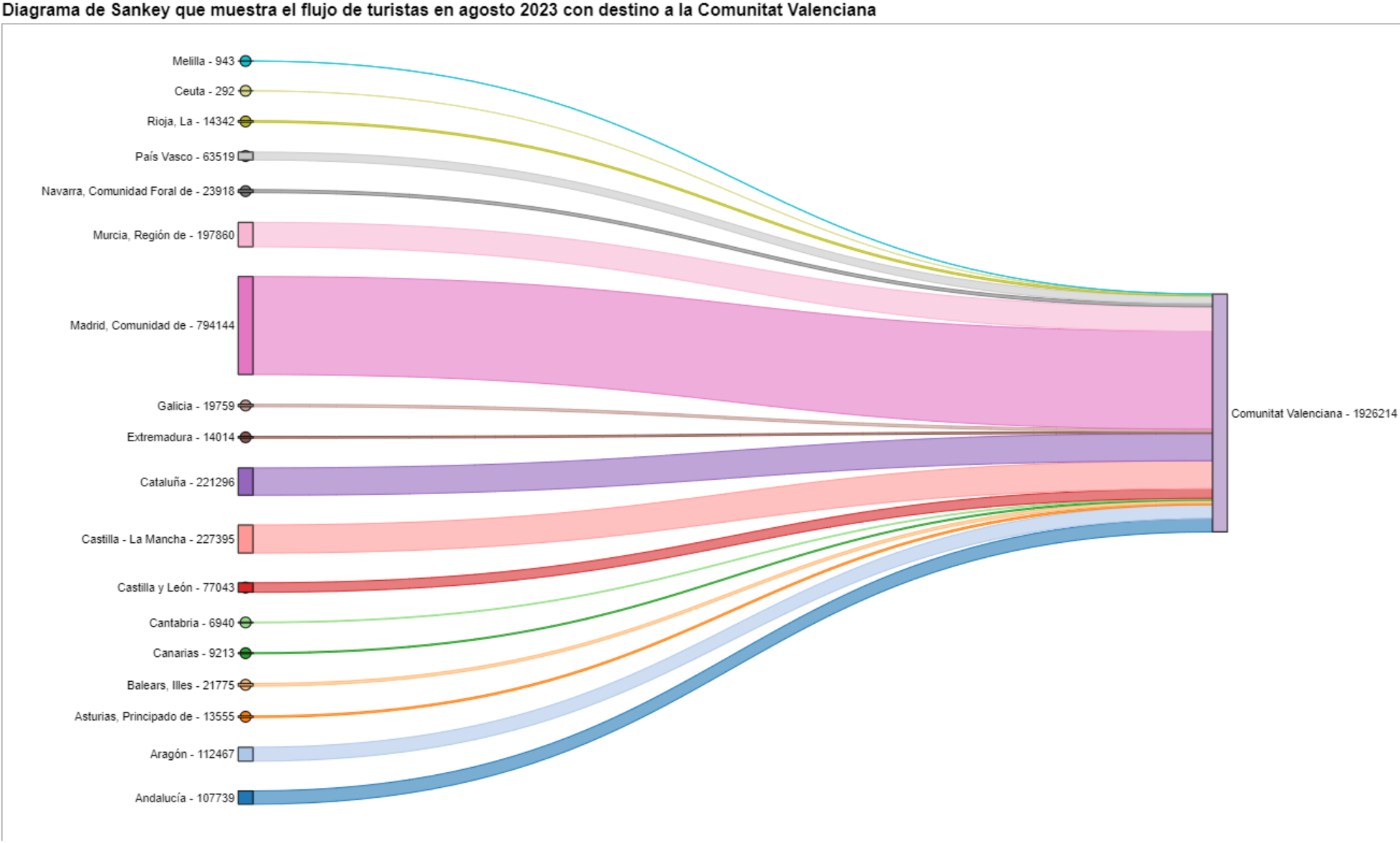
For the Sankey diagrams, we will focus on the Valencian Community, as it is a popular holiday destination. We filter the edges we created for the previous chord diagram so that they only contain flows that end in the Valencian Community. The same procedure could be applied to study any other CA or could be inverted to analyze where Valencians go on vacation. We visualize the Sankey diagram which, like the chord diagrams, is interactive within the notebook. The visual aspect would be like this:
Figure 9. Sankey diagram showing the flow of tourists in August 2023 destined for the Valencian Community.
As we could already intuit from the chord diagram above, see Figure 8, the largest group of tourists arriving in the Valencian Community comes from Madrid. We also see that there is a high number of tourists visiting the Valencian Community from neighboring CCAA such as Murcia, Andalucía, and Catalonia.
To verify that these trends occur in the three provinces of the Valencian Community, we are going to create a Sankey diagram that shows on the left margin all the CCAA and on the right margin the three provinces of the Valencian Community.
To create this Sankey diagram at the provincial level, we have to filter our initial pandas.DataFrame to extract the relevant information from it. The steps in the notebook can be adapted to perform this analysis at the provincial level for any other CA. Although we are not reusing the function we used previously, we can also change the analysis period.
The Sankey diagram that visualizes the tourist flows that arrived in August 2023 to the three Valencian provinces would look like this:
Figure 10. Sankey diagram August 2023 showing the flow of tourists destined for provinces of the Valencian Community.
We can observe that, as we already assumed, the largest number of tourists arriving in the Valencian Community in August comes from the Community of Madrid. However, we can verify that this is not true for the province of Castellón, where in August 2023 the majority of tourists were Valencians who traveled within their own CA.
6. Conclusions of the exercise
Thanks to the visualization techniques used in this exercise, we have been able to observe the tourist flows that move within the national territory, focusing on making comparisons between different times of the year and trying to identify patterns. In both the chord diagrams and the Sankey diagrams that we have created, we have been able to observe the influx of Madrilenian tourists on the Valencian coasts in summer. We have also been able to identify the autonomous communities where tourists leave their own autonomous community the least, such as Catalonia and Andalucía.
7. Do you want to do the exercise?
We invite the reader to execute the code contained in the Google Colab notebook that accompanies this exercise to continue with the analysis of tourist flows. We leave here some ideas of possible questions and how they could be answered:
The impact of the pandemic: we have already mentioned it briefly above, but an interesting question would be to measure the impact that the coronavirus pandemic has had on tourism. We can compare the data from previous years with 2020 and also analyze the following years to detect stabilization trends. Given that the function we have created allows easily changing the time period under analysis, we suggest you do this analysis on your own.
Time intervals: it is also possible to modify the function we have been using in such a way that it not only allows selecting a specific time period, but also allows time intervals.
Provincial level analysis: likewise, an advanced reader with Pandas can challenge themselves to create a Sankey diagram that visualizes which provinces the inhabitants of a certain region travel to, for example, Ourense. In order not to have too many destination provinces that could make the Sankey diagram illegible, only the 10 most visited could be visualized. To obtain the data to create this visualization, the reader would have to play with the filters they apply to the dataset and with the groupby method of pandas, being inspired by the already executed code.
We hope that this practical exercise has provided you with sufficient knowledge to develop your own visualizations. If you have any data science topic that you would like us to cover soon, do not hesitate to propose your interest through our contact channels.
In addition, remember that you have more exercises available in the section "Data science exercises".
Environment
Energy
Industry
1. Introduction
In the information age, artificial intelligence has proven to be an invaluable tool for a variety of applications. One of the most incredible manifestations of this technology is GPT (Generative Pre-trained Transformer), developed by OpenAI. GPT is a natural language model that can understand and generate text, providing coherent and contextually relevant responses. With the recent introduction of Chat GPT-4, the capabilities of this model have been further expanded, allowing for greater customisation and adaptability to different themes.
In this post, we will show you how to set up and customise a specialised critical minerals wizard using GPT-4 and open data sources. As we have shown in previous publications critical minerals are fundamental to numerous industries, including technology, energy and defence, due to their unique properties and strategic importance. However, information on these materials can be complex and scattered, making a specialised assistant particularly useful.
The aim of this post is to guide you step by step from the initial configuration to the implementation of a GPT wizard that can help you to solve doubts and provide valuable information about critical minerals in your day to day life. In addition, we will explore how to customise aspects of the assistant, such as the tone and style of responses, to perfectly suit your needs. At the end of this journey, you will have a powerful, customised tool that will transform the way you access and use critical open mineral information.
Access the data lab repository on Github
2. Context
The transition to a sustainable future involves not only changes in energy sources, but also in the material resources we use. The success of sectors such as energy storage batteries, wind turbines, solar panels, electrolysers, drones, robots, data transmission networks, electronic devices or space satellites depends heavily on access to the raw materials critical to their development. We understand that a mineral is critical when the following factors are met:
Its global reserves are scarce
There are no alternative materials that can perform their function (their properties are unique or very unique)
They are indispensable materials for key economic sectors of the future, and/or their supply chain is high risk
You can learn more about critical minerals in the post mentioned above.
3. Target
This exercise focuses on showing the reader how to customise a specialised GPT model for a specific use case. We will adopt a "learning-by-doing" approach, so that the reader can understand how to set up and adjust the model to solve a real and relevant problem, such as critical mineral expert advice. This hands-on approach not only improves understanding of language model customisation techniques, but also prepares readers to apply this knowledge to real-world problem solving, providing a rich learning experience directly applicable to their own projects.
The GPT assistant specialised in critical minerals will be designed to become an essential tool for professionals, researchers and students. Its main objective will be to facilitate access to accurate and up-to-date information on these materials, to support strategic decision-making and to promote education in this field. The following are the specific objectives we seek to achieve with this assistant:
Provide accurate and up-to-date information:
The assistant should provide detailed and accurate information on various critical minerals, including their composition, properties, industrial uses and availability.
Keep up to date with the latest research and market trends in the field of critical minerals.
Assist in decision-making:
To provide data and analysis that can assist strategic decision making in industry and critical minerals research.
Provide comparisons and evaluations of different minerals in terms of performance, cost and availability.
Promote education and awareness of the issue:
Act as an educational tool for students, researchers and practitioners, helping to improve their knowledge of critical minerals.
Raise awareness of the importance of these materials and the challenges related to their supply and sustainability.
4. Resources
To configure and customise our GPT wizard specialising in critical minerals, it is essential to have a number of resources to facilitate implementation and ensure the accuracy and relevance of the model''s responses. In this section, we will detail the necessary resources that include both the technological tools and the sources of information that will be integrated into the assistant''s knowledge base.
Tools and Technologies
The key tools and technologies to develop this exercise are:
OpenAI account: required to access the platform and use the GPT-4 model. In this post, we will use ChatGPT''s Plus subscription to show you how to create and publish a custom GPT. However, you can develop this exercise in a similar way by using a free OpenAI account and performing the same set of instructions through a standard ChatGPT conversation.
Microsoft Excel: we have designed this exercise so that anyone without technical knowledge can work through it from start to finish. We will only use office tools such as Microsoft Excel to make some adjustments to the downloaded data.
In a complementary way, we will use another set of tools that will allow us to automate some actions without their use being strictly necessary:
Google Colab: is a Python Notebooks environment that runs in the cloud, allowing users to write and run Python code directly in the browser. Google Colab is particularly useful for machine learning, data analysis and experimentation with language models, offering free access to powerful computational resources and facilitating collaboration and project sharing.
Markmap: is a tool that visualises Markdown mind maps in real time. Users write ideas in Markdown and the tool renders them as an interactive mind map in the browser. Markmap is useful for project planning, note taking and organising complex information visually. It facilitates understanding and the exchange of ideas in teams and presentations.
Sources of information
Raw Materials Information System (RMIS): raw materials information system maintained by the Joint Research Center of the European Union. It provides detailed and up-to-date data on the availability, production and consumption of raw materials in Europe.
International Energy Agency (IEA) Catalogue of Reports and Data: the International Energy Agency (IEA) offers a comprehensive catalogue of energy-related reports and data, including statistics on production, consumption and reserves of energy and critical minerals.
Mineral Database of the Spanish Geological and Mining Institute (BDMIN in its acronym in Spanish): contains detailed information on minerals and mineral deposits in Spain, useful to obtain specific data on the production and reserves of critical minerals in the country.
With these resources, you will be well equipped to develop a specialised GPT assistant that can provide accurate and relevant answers on critical minerals, facilitating informed decision-making in the field.
5. Development of the exercise
5.1. Building the knowledge base
For our specialised critical minerals GPT assistant to be truly useful and accurate, it is essential to build a solid and structured knowledge base. This knowledge base will be the set of data and information that the assistant will use to answer queries. The quality and relevance of this information will determine the effectiveness of the assistant in providing accurate and useful answers.
Search for Data Sources
We start with the collection of information sources that will feed our knowledge base. Not all sources of information are equally reliable. It is essential to assess the quality of the sources identified, ensuring that:
Information is up to date: the relevance of data can change rapidly, especially in dynamic fields such as critical minerals.
The source is reliable and recognised: it is necessary to use sources from recognised and respected academic and professional institutions.
Data is complete and accessible: it is crucial that data is detailed and accessible for integration into our wizard.
In our case, we developed an online search in different platforms and information repositories trying to select information belonging to different recognised entities:
Research centres and universities:
They publish detailed studies and reports on the research and development of critical minerals.
Example: RMIS of the Joint Research Center of the European Union.
Governmental institutions and international organisations:
These entities usually provide comprehensive and up-to-date data on the availability and use of critical minerals.
Example: International Energy Agency (IEA).
Specialised databases:
They contain technical and specific data on deposits and production of critical minerals.
Example: Minerals Database of the Spanish Geological and Mining Institute (BDMIN).
Selection and preparation of information
We will now focus on the selection and preparation of existing information from these sources to ensure that our GPT assistant can access accurate and useful data.
RMIS of the Joint Research Center of the European Union:
Selected information:
We selected the report "Supply chain analysis and material demand forecast in strategic technologies and sectors in the EU - A foresight study". This is an analysis of the supply chain and demand for minerals in strategic technologies and sectors in the EU. It presents a detailed study of the supply chains of critical raw materials and forecasts the demand for minerals up to 2050.
Necessary preparation:
The format of the document, PDF, allows the direct ingestion of the information by our assistant. However, as can be seen in Figure 1, there is a particularly relevant table on pages 238-240 which analyses, for each mineral, its supply risk, typology (strategic, critical or non-critical) and the key technologies that employ it. We therefore decided to extract this table into a structured format (CSV), so that we have two pieces of information that will become part of our knowledge base.
Figure 1: Table of minerals contained in the JRC PDF
To programmatically extract the data contained in this table and transform it into a more easily processable format, such as CSV(comma separated values), we will use a Python script that we can use through the platform Google Colab platform (Figure 2).
Figure 2: Script Python para la extracción de datos del PDF de JRC desarrollado en plataforma Google Colab.
To summarise, this script:
It is based on the open source library PyPDF2capable of interpreting information contained in PDF files.
First, it extracts in text format (string) the content of the pages of the PDF where the mineral table is located, removing all the content that does not correspond to the table itself.
It then goes through the string line by line, converting the values into columns of a data table. We will know that a mineral is used in a key technology if in the corresponding column of that mineral we find a number 1 (otherwise it will contain a 0).
Finally, it exports the table to a CSV file for further use.
International Energy Agency (IEA):
Selected information:
We selected the report "Global Critical Minerals Outlook 2024". It provides an overview of industrial developments in 2023 and early 2024, and offers medium- and long-term prospects for the demand and supply of key minerals for the energy transition. It also assesses risks to the reliability, sustainability and diversity of critical mineral supply chains.
Necessary preparation:
The format of the document, PDF, allows us to ingest the information directly by our virtual assistant. In this case, we will not make any adjustments to the selected information.
Spanish Geological and Mining Institute''s Minerals Database (BDMIN)
Selected information:
In this case, we use the form to select the existing data in this database for indications and deposits in the field of metallogeny, in particular those with lithium content.
Figure 3: Dataset selection in BDMIN.
Necessary preparation:
We note how the web tool allows online visualisation and also the export of this data in various formats. Select all the data to be exported and click on this option to download an Excel file with the desired information.
Figure 4: Visualization and download tool in BDMIN
Figure 5: BDMIN Downloaded Data.
All the files that make up our knowledge base can be found at GitHub, so that the reader can skip the downloading and preparation phase of the information.
5.2. GPT configuration and customisation for critical minerals
When we talk about "creating a GPT," we are actually referring to the configuration and customisation of a GPT (Generative Pre-trained Transformer) based language model to suit a specific use case. In this context, we are not creating the model from scratch, but adjusting how the pre-existing model (such as OpenAI''s GPT-4) interacts and responds within a specific domain, in this case, on critical minerals.
First of all, we access the application through our browser and, if we do not have an account, we follow the registration and login process on the ChatGPT platform. As mentioned above, in order to create a GPT step-by-step, you will need to have a Plus account. However, readers who do not have such an account can work with a free account by interacting with ChatGPT through a standard conversation.
Figure 6: ChatGPT login and registration page.
Once logged in, select the "Explore GPT" option, and then click on "Create" to begin the process of creating your GPT.
Figure 7: Creation of new GPT.
The screen will display the split screen for creating a new GPT: on the left, we will be able to talk to the system to indicate the characteristics that our GPT should have, while on the left we will be able to interact with our GPT to validate that its behaviour is adequate as we go through the configuration process.
Figure 8: Screen of creating new GPT.
In the GitHub of this project, we can find all the prompts or instructions that we will use to configure and customise our GPT and that we will have to introduce sequentially in the "Create" tab, located on the left tab of our screens, to complete the steps detailed below.
The steps we will follow for the creation of the GPT are as follows:
First, we will outline the purpose and basic considerations for our GPT so that you can understand how to use it.
Figure 9: Basic instructions for new GPT.
2. We will then create a name and an image to represent our GPT and make it easily identifiable. In our case, we will call it MateriaGuru.
Figure 10: Name selection for new GPT.
Figure 11: Image creation for GPT.
3.We will then build the knowledge base from the information previously selected and prepared to feed the knowledge of our GPT.
Figure 12: Uploading of information to the new GPT knowledge base.
4. Now, we can customise conversational aspects such as their tone, the level of technical complexity of their response or whether we expect brief or elaborate answers.
5. Lastly, from the "Configure" tab, we can indicate the conversation starters desired so that users interacting with our GPT have some ideas to start the conversation in a predefined way.
Figure 13: Configure GPT tab.
In Figure 13 we can also see the final result of our training, where key elements such as their image, name, instructions, conversation starters or documents that are part of their knowledge base appear.
5.3. Validation and publication of GPT
Before we sign off our new GPT-based assistant, we will proceed with a brief validation of its correct configuration and learning with respect to the subject matter around which we have trained it. For this purpose, we prepared a battery of questions that we will ask MateriaGuru to check that it responds appropriately to a real scenario of use.
#
Question
Answer
1
Which critical minerals have experienced a significant drop in prices in 2023?
Battery mineral prices saw particularly large drops with lithium prices falling by 75% and cobalt, nickel and graphite prices falling by between 30% and 45%.
2
What percentage of global solar photovoltaic (PV) capacity was added by China in 2023?
China accounted for 62% of the increase in global solar PV capacity in 2023.
3
What is the scenario that projects electric car (EV) sales to reach 65% by 2030?
The Net Zero Emissions (NZE) scenario for 2050 projects that electric car sales will reach 65% by 2030.
4
What was the growth in lithium demand in 2023?
Lithium demand increased by 30% in 2023.
5
Which country was the largest electric car market in 2023?
China was the largest electric car market in 2023 with 8.1 million electric car sales representing 60% of the global total.
6
What is the main risk associated with market concentration in the battery graphite supply chain?
More than 90% of battery-grade graphite and 77% of refined rare earths in 2030 originate in China, posing a significant risk to market concentration.
7
What proportion of global battery cell production capacity was in China in 2023?
China owned 85% of battery cell production capacity in 2023.
8
How much did investment in critical minerals mining increase in 2023?
Investment in critical minerals mining grew by 10% in 2023.
9
What percentage of battery storage capacity in 2023 was composed of lithium iron phosphate (LFP) batteries?
By 2023, LFP batteries would constitute approximately 80% of the total battery storage market.
10
What is the forecast for copper demand in a net zero emissions (NZE) scenario for 2040?
In the net zero emissions (NZE) scenario for 2040, copper demand is expected to have the largest increase in terms of production volume.
Figure 14: Table with battery of questions for the validation of our GPT.
Using the preview section on the right-hand side of our screens, we launch the battery of questions and validate that the answers correspond to those expected.
Figure 15: Validation of GPT responses.
Finally, click on the "Create" button to finalise the process. We will be able to select between different alternatives to restrict its use by other users.
Figure 16: Publication of our GPT.
6. Scenarios of use
In this section we show several scenarios in which we can take advantage of MateriaGuru in our daily life. On the GitHub of the project you can find the prompts used to replicate each of them.
6.1. Consultation of critical minerals information
The most typical scenario for the use of this type of GPTs is assistance in resolving doubts related to the topic in question, in this case, critical minerals. As an example, we have prepared a set of questions that the reader can pose to the GPT created to understand in more detail the relevance and current status of a critical material such as graphite from the reports provided to our GPT.
Figure 17: Resolution of critical mineral queries.
We can also ask you specific questions about the tabulated information provided on existing sites and evidence on Spanish territory.
Figure 18: Lithium reserves in Extremadura.
6.2. Representation of quantitative data visualisations
Another common scenario is the need to consult quantitative information and make visual representations for better understanding. In this scenario, we can see how MateriaGuru is able to generate an interactive visualisation of graphite production in tonnes for the main producing countries.
Figure 19: Interactive visualisation generation with our GPT.
6.3. Generating mind maps to facilitate understanding
Finally, in line with the search for alternatives for a better access and understanding of the existing knowledge in our GPT, we will propose to MateriaGuru the construction of a mind map that allows us to understand in a visual way key concepts of critical minerals. For this purpose, we use the open Markmap notation (Markdown Mindmap), which allows us to define mind maps using markdown notation.
Figure 20: Generation of mind maps from our GPT
We will need to copy the generated code and enter it in a markmapviewer in order to generate the desired mind map. We facilitate here a version of this code generated by MateriaGuru.
Figure 21: Visualisation of mind maps.
7. Results and conclusions
In the exercise of building an expert assistant using GPT-4, we have succeeded in creating a specialised model for critical minerals. This wizard provides detailed and up-to-date information on critical minerals, supporting strategic decision making and promoting education in this field. We first gathered information from reliable sources such as the RMIS, the International Energy Agency (IEA), and the Spanish Geological and Mining Institute (BDMIN). We then process and structure the data appropriately for integration into the model. Validations showed that the wizard accurately answers domain-relevant questions, facilitating access to your information.
In this way, the development of the specialised critical minerals assistant has proven to be an effective solution for centralising and facilitating access to complex and dispersed information.
The use of tools such as Google Colab and Markmap has enabled better organisation and visualisation of data, increasing efficiency in knowledge management. This approach not only improves the understanding and use of critical mineral information, but also prepares users to apply this knowledge in real-world contexts.
The practical experience gained in this exercise is directly applicable to other projects that require customisation of language models for specific use cases.
8. Do you want to do the exercise?
If you want to replicate this exercise, access this this repository where you will find more information (the prompts used, the code generated by MateriaGuru, etc.)
Also, remember that you have at your disposal more exercises in the section "Step-by-step visualisations".
Content elaborated by Juan Benavente, industrial engineer and expert in technologies linked to the data economy. The contents and points of view reflected in this publication are the sole responsibility of the author.
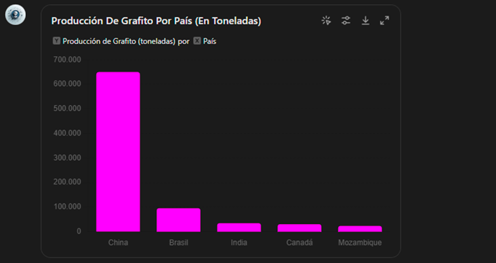
Environment
Transport
Economy
1. Introduction
Visualisations are graphical representations of data that allow to communicate, in a simple and effective way, the information linked to the data. The visualisation possibilities are very wide ranging, from basic representations such as line graphs, bar charts or relevant metrics, to interactive dashboards.
In this section of "Step-by-Step Visualisations we are regularly presenting practical exercises making use of open data available at datos.gob.es or other similar catalogues. They address and describe in a simple way the steps necessary to obtain the data, carry out the relevant transformations and analyses, and finally draw conclusions, summarizing the information.
Documented code developments and free-to-use tools are used in each practical exercise. All the material generated is available for reuse in the GitHub repository of datos.gob.es.
In this particular exercise, we will explore the current state of electric vehicle penetration in Spain and the future prospects for this disruptive technology in transport.
Access the data lab repository on Github
Run the data pre-processing code on Google Colab
In this video (available with English subtitles), the author explains what you will find both on Github and Google Colab.
2. Context: why is the electric vehicle important?
The transition towards more sustainable mobility has become a global priority, placing the electric vehicle (EV) at the centre of many discussions on the future of transport. In Spain, this trend towards the electrification of the car fleet not only responds to a growing consumer interest in cleaner and more efficient technologies, but also to a regulatory and incentive framework designed to accelerate the adoption of these vehicles. With a growing range of electric models available on the market, electric vehicles represent a key part of the country's strategy to reduce greenhouse gas emissions, improve urban air quality and foster technological innovation in the automotive sector.
However, the penetration of EVs in the Spanish market faces a number of challenges, from charging infrastructure to consumer perception and knowledge of EVs. Expansion of the freight network, together with supportive policies and fiscal incentives, are key to overcoming existing barriers and stimulating demand. As Spain moves towards its sustainability and energy transition goals, analysing the evolution of the electric vehicle market becomes an essential tool to understand the progress made and the obstacles that still need to be overcome.
3. Objective
This exercise focuses on showing the reader techniques for the processing, visualisation and advanced analysis of open data using Python. We will adopt a "learning-by-doing" approach so that the reader can understand the use of these tools in the context of solving a real and topical challenge such as the study of EV penetration in Spain. This hands-on approach not only enhances understanding of data science tools, but also prepares readers to apply this knowledge to solve real problems, providing a rich learning experience that is directly applicable to their own projects.
The questions we will try to answer through our analysis are:
Which vehicle brands led the market in 2023?
Which vehicle models were the best-selling in 2023?
What market share will electric vehicles absorb in 2023?
Which electric vehicle models were the best-selling in 2023?
How have vehicle registrations evolved over time?
Are we seeing any trends in electric vehicle registrations?
How do we expect electric vehicle registrations to develop next year?
How much CO2 emission reduction can we expect from the registrations achieved over the next year?
4. Resources
To complete the development of this exercise we will require the use of two categories of resources: Analytical Tools and Datasets.
4.1. Dataset
To complete this exercise we will use a dataset provided by the Dirección General de Tráfico (DGT) through its statistical portal, also available from the National Open Data catalogue (datos.gob.es). The DGT statistical portal is an online platform aimed at providing public access to a wide range of data and statistics related to traffic and road safety. This portal includes information on traffic accidents, offences, vehicle registrations, driving licences and other relevant data that can be useful for researchers, industry professionals and the general public.
In our case, we will use their dataset of vehicle registrations in Spain available via:
Open Data Catalogue of the Spanish Government.
Statistical portal of the DGT.
Although during the development of the exercise we will show the reader the necessary mechanisms for downloading and processing, we include pre-processed data
in the associated GitHub repository, so that the reader can proceed directly to the analysis of the data if desired.
*The data used in this exercise were downloaded on 04 March 2024. The licence applicable to this dataset can be found at https://datos.gob.es/avisolegal.
4.2. Analytical tools
Programming language: Python - a programming language widely used in data analysis due to its versatility and the wide range of libraries available. These tools allow users to clean, analyse and visualise large datasets efficiently, making Python a popular choice among data scientists and analysts.
Platform: Jupyter Notebooks - ia web application that allows you to create and share documents containing live code, equations, visualisations and narrative text. It is widely used for data science, data analytics, machine learning and interactive programming education.
Main libraries and modules:
Data manipulation: Pandas - an open source library that provides high-performance, easy-to-use data structures and data analysis tools.
Data visualisation:
Matplotlib: a library for creating static, animated and interactive visualisations in Python..
Seaborn: a library based on Matplotlib. It provides a high-level interface for drawing attractive and informative statistical graphs.
Statistics and algorithms:
Statsmodels: a library that provides classes and functions for estimating many different statistical models, as well as for testing and exploring statistical data.
Pmdarima: a library specialised in automatic time series modelling, facilitating the identification, fitting and validation of models for complex forecasts.
5. Exercise development
It is advisable to run the Notebook with the code at the same time as reading the post, as both didactic resources are complementary in future explanations
The proposed exercise is divided into three main phases.
5.1 Initial configuration
This section can be found in point 1 of the Notebook.
In this short first section, we will configure our Jupyter Notebook and our working environment to be able to work with the selected dataset. We will import the necessary Python libraries and create some directories where we will store the downloaded data.
5.2 Data preparation
This section can be found in point 2 of the Notebookk.
All data analysis requires a phase of accessing and processing to obtain the appropriate data in the desired format. In this phase, we will download the data from the statistical portal and transform it into the format Apache Parquet format before proceeding with the analysis.
Those users who want to go deeper into this task, please read this guide Practical Introductory Guide to Exploratory Data Analysis.
5.3 Data analysis
This section can be found in point 3 of the Notebook.
5.3.1 Análisis descriptivo
In this third phase, we will begin our data analysis. To do so,we will answer the first questions using datavisualisation tools to familiarise ourselves with the data. Some examples of the analysis are shown below:
Top 10 Vehicles registered in 2023: In this visualisation we show the ten vehicle models with the highest number of registrations in 2023, also indicating their combustion type. The main conclusions are:
The only European-made vehicles in the Top 10 are the Arona and the Ibiza from Spanish brand SEAT. The rest are Asians.
Nine of the ten vehicles are powered by gasoline.
The only vehicle in the Top 10 with a different type of propulsion is the DACIA Sandero LPG (Liquefied Petroleum Gas).
Figure 1. Graph "Top 10 vehicles registered in 2023"
Market share by propulsion type: In this visualisation we represent the percentage of vehicles registered by each type of propulsion (petrol, diesel, electric or other). We see how the vast majority of the market (>70%) was taken up by petrol vehicles, with diesel being the second choice, and how electric vehicles reached 5.5%.
Figure 2. Graph "Market share by propulsion type".
Historical development of registrations: This visualisation represents the evolution of vehicle registrations over time. It shows the monthly number of registrations between January 2015 and December 2023 distinguishing between the propulsion types of the registered vehicles, and there are several interesting aspects of this graph:
We observe an annual seasonal behaviour, i.e. we observe patterns or variations that are repeated at regular time intervals. We see recurring high levels of enrolment in June/July, while in August/September they decrease drastically. This is very relevant, as the analysis of time series with a seasonal factor has certain particularities.
The huge drop in registrations during the first months of COVID is also very remarkable.
We also see that post-covid enrolment levels are lower than before.
Finally, we can see how between 2015 and 2023 the registration of electric vehicles is gradually increasing.
Figure 3. Graph "Vehicle registrations by propulsion type".
Trend in the registration of electric vehicles: We now analyse the evolution of electric and non-electric vehicles separately using heat maps as a visual tool. We can observe very different behaviours between the two graphs. We observe how the electric vehicle shows a trend of increasing registrations year by year and, despite the COVID being a halt in the registration of vehicles, subsequent years have maintained the upward trend.
Figure 4. Graph "Trend in registration of conventional vs. electric vehicles".
5.3.2. Predictive analytics
To answer the last question objectively, we will use predictive models that allow us to make estimates regarding the evolution of electric vehicles in Spain. As we can see, the model constructed proposes a continuation of the expected growth in registrations throughout the year of 70,000, reaching values close to 8,000 registrations in the month of December 2024 alone.
Figure 5. Graph "Predicted electric vehicle registrations".
5. Conclusions
As a conclusion of the exercise, we can observe, thanks to the analysis techniques used, how the electric vehicle is penetrating the Spanish vehicle fleet at an increasing speed, although it is still at a great distance from other alternatives such as diesel or petrol, for now led by the manufacturer Tesla. We will see in the coming years whether the pace grows at the level needed to meet the sustainability targets set and whether Tesla remains the leader despite the strong entry of Asian competitors.
6. Do you want to do the exercise?
If you want to learn more about the Electric Vehicle and test your analytical skills, go to this code repository where you can develop this exercise step by step.
Also, remember that you have at your disposal more exercises in the section "Step by step visualisations" "Step-by-step visualisations" section.
Content elaborated by Juan Benavente, industrial engineer and expert in technologies linked to the data economy. The contents and points of view reflected in this publication are the sole responsibility of the author.
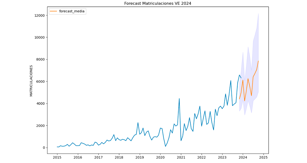
Energy
Science and technology
Town planning and infrastructures
1. Introduction
Visualizations are graphical representations of data that allow you to communicate, in a simple and effective way, the information linked to it. The visualization possibilities are very extensive, from basic representations such as line graphs, bar graphs or relevant metrics, to visualizations configured on interactive dashboards.
In the section of “Step-by-step visualizations” we are periodically presenting practical exercises making use of open data available in datos.gob.es or other similar catalogs. They address and describe in a simple way the steps necessary to obtain the data, carry out the transformations and analyses that are pertinent to finally obtain conclusions as a summary of this information.
In each of these hands-on exercises, conveniently documented code developments are used, as well as free-to-use tools. All generated material is available for reuse in the datos.gob.es GitHub repository.
Accede al repositorio del laboratorio de datos en Github.
Ejecuta el código de pre-procesamiento de datos sobre Google Colab.
2. Objetive
The main objective of this exercise is to show how to carry out, in a didactic way, a predictive analysis of time series based on open data on electricity consumption in the city of Barcelona. To do this, we will carry out an exploratory analysis of the data, define and validate the predictive model, and finally generate the predictions together with their corresponding graphs and visualizations.
Predictive time series analytics are statistical and machine learning techniques used to forecast future values in datasets that are collected over time. These predictions are based on historical patterns and trends identified in the time series, with their primary purpose being to anticipate changes and events based on past data.
The initial open dataset consists of records from 2019 to 2022 inclusive, on the other hand, the predictions will be made for the year 2023, for which we do not have real data.
Once the analysis has been carried out, we will be able to answer questions such as the following:
What is the future prediction of electricity consumption?
How accurate has the model been with the prediction of already known data?
Which days will have maximum and minimum consumption based on future predictions?
Which months will have a maximum and minimum average consumption according to future predictions?
These and many other questions can be solved through the visualizations obtained in the analysis, which will show the information in an orderly and easy-to-interpret way.
3. Resources
3.1. Datasets
The open datasets used contain information on electricity consumption in the city of Barcelona in recent years. The information they provide is the consumption in (MWh) broken down by day, economic sector, zip code and time slot.
These open datasets are published by Barcelona City Council in the datos.gob.es catalogue, through files that collect the records on an annual basis. It should be noted that the publisher updates these datasets with new records frequently, so we have used only the data provided from 2019 to 2022 inclusive.
Series anuales de consumo eléctrico (MWh) en la ciudad de Barcelona.
These datasets are also available for download from the following Github repository.
3.2. Tools
To carry out the analysis, the Python programming language written on a Jupyter Notebook hosted in the Google Colab cloud service has been used.
"Google Colab" or, also called Google Colaboratory, is a cloud service from Google Research that allows you to program, execute and share code written in Python or R on top of a Jupyter Notebook from your browser, so it requires no configuration. This service is free of charge.
The Looker Studio tool was used to create the interactive visualizations.
"Looker Studio", formerly known as Google Data Studio, is an online tool that allows you to make interactive visualizations that can be inserted into websites or exported as files.
If you want to know more about tools that can help you in data processing and visualization, you can refer to the "Data processing and visualization tools" report.
4. Predictive time series analysis
Predictive time series analysis is a technique that uses historical data to predict future values of a variable that changes over time. Time series is data that is collected at regular intervals, such as days, weeks, months, or years. It is not the purpose of this exercise to explain in detail the characteristics of time series, as we focus on briefly explaining the prediction model. However, if you want to know more about it, you can consult the following manual.
This type of analysis assumes that the future values of a variable will be correlated with historical values. Using statistical and machine learning techniques, patterns in historical data can be identified and used to predict future values.
The predictive analysis carried out in the exercise has been divided into five phases; data preparation, exploratory data analysis, model training, model validation, and prediction of future values), which will be explained in the following sections.
The processes described below are developed and commented on in the following Notebook executable from Google Colab along with the source code that is available in our Github account.
It is advisable to run the Notebook with the code at the same time as reading the post, since both didactic resources are complementary in future explanations.
4.1 Data preparation
This section can be found in point 1 of the Notebook.
In this section, the open datasets described in the previous points that we will use in the exercise are imported, paying special attention to obtaining them and validating their content, ensuring that they are in the appropriate and consistent format for processing and that they do not contain errors that could condition future steps.
4.2 Exploratory Data Analysis (EDA)
This section can be found in point 2 of the Notebook.
In this section we will carry out an exploratory data analysis (EDA), in order to properly interpret the source data, detect anomalies, missing data, errors or outliers that could affect the quality of subsequent processes and results.
Then, in the following interactive visualization, you will be able to inspect the data table with the historical consumption values generated in the previous point, being able to filter by specific period. In this way, we can visually understand the main information in the data series.
Once you have inspected the interactive visualization of the time series, you will have observed several values that could potentially be considered outliers, as shown in the figure below. We can also numerically calculate these outliers, as shown in the notebook.
Figure 1. Time Series Outliers with Historical Data
Once the outliers have been evaluated, for this year it has been decided to modify only the one registered on the date "2022-12-05". To do this, the value will be replaced by the average of the value recorded the previous day and the day after.
The reason for not eliminating the rest of the outliers is because they are values recorded on consecutive days, so it is assumed that they are correct values affected by external variables that are beyond the scope of the exercise. Once the problem detected with the outliers has been solved, this will be the time series of data that we will use in the following sections.
Figure 2. Time series of historical data after outliers have been processed.
If you want to know more about these processes, you can refer to the Practical Guide to Introduction to Exploratory Data Analysis.
4.3 Model training
This section can be found in point 3 of the Notebook.
First, we create within the data table the temporal attributes (year, month, day of the week, and quarter). These attributes are categorical variables that help ensure that the model is able to accurately capture the unique characteristics and patterns of these variables. Through the following box plot visualizations, we can see their relevance within the time series values.
Figure 3. Box Diagrams of Generated Temporal Attributes
We can observe certain patterns in the charts above, such as the following:
Weekdays (Monday to Friday) have a higher consumption than on weekends.
The year with the lowest consumption values is 2020, which we understand is due to the reduction in service and industrial activity during the pandemic.
The month with the highest consumption is July, which is understandable due to the use of air conditioners.
The second quarter is the one with the lowest consumption values, with April standing out as the month with the lowest values.
Next, we divide the data table into training set and validation set. The training set is used to train the model, i.e., the model learns to predict the value of the target variable from that set, while the validation set is used to evaluate the performance of the model, i.e., the model is evaluated against the data from that set to determine its ability to predict the new values.
This splitting of the data is important to avoid overfitting, with the typical proportion of the data used for the training set being 70% and the validation set being approximately 30%. For this exercise we have decided to generate the training set with the data between "01-01-2019" to "01-10-2021", and the validation set with those between "01-10-2021" and "31-12-2022" as we can see in the following graph.
Figure 4. Historical data time series divided into training set and validation set
For this type of exercise, we have to use some regression algorithm. There are several models and libraries that can be used for time series prediction. In this exercise we will use the "Gradient Boosting" model, a supervised regression model that is a machine learning algorithm used to predict a continuous value based on the training of a dataset containing known values for the target variable (in our example the variable "value") and the values of the independent variables (in our exercise the temporal attributes).
It is based on decision trees and uses a technique called "boosting" to improve the accuracy of the model, being known for its efficiency and ability to handle a variety of regression and classification problems.
Its main advantages are the high degree of accuracy, robustness and flexibility, while some of its disadvantages are its sensitivity to outliers and that it requires careful optimization of parameters.
We will use the supervised regression model offered in the XGBBoost library, which can be adjusted with the following parameters:
n_estimators: A parameter that affects the performance of the model by indicating the number of trees used. A larger number of trees generally results in a more accurate model, but it can also take more time to train.
early_stopping_rounds: A parameter that controls the number of training rounds that will run before the model stops if performance in the validation set does not improve.
learning_rate: Controls the learning speed of the model. A higher value will make the model learn faster, but it can lead to overfitting.
max_depth: Control the maximum depth of trees in the forest. A higher value can provide a more accurate model, but it can also lead to overfitting.
min_child_weight: Control the minimum weight of a sheet. A higher value can help prevent overfitting.
Gamma: Controls the amount of expected loss reduction needed to split a node. A higher value can help prevent overfitting.
colsample_bytree: Controls the proportion of features that are used to build each tree. A higher value can help prevent overfitting.
Subsample: Controls the proportion of the data that is used to construct each tree. A higher value can help prevent overfitting.
These parameters can be adjusted to improve model performance on a specific dataset. It's a good idea to experiment with different values of these parameters to find the value that provides the best performance in your dataset.
Finally, by means of a bar graph, we will visually observe the importance of each of the attributes during the training of the model. It can be used to identify the most important attributes in a dataset, which can be useful for model interpretation and feature selection.
Figure 5. Bar Chart with Importance of Temporal Attributes
4.4 Model training
This section can be found in point 4 of the Notebook.
Once the model has been trained, we will evaluate how accurate it is for the known values in the validation set.
We can visually evaluate the model by plotting the time series with the known values along with the predictions made for the validation set as shown in the figure below.
Figure 6. Time series with validation set data next to prediction data.
We can also numerically evaluate the accuracy of the model using different metrics. In this exercise, we have chosen to use the mean absolute percentage error (ASM) metric, which has been 6.58%. The accuracy of the model is considered high or low depending on the context and expectations in such a model, generally an ASM is considered low when it is less than 5%, while it is considered high when it is greater than 10%. In this exercise, the result of the model validation can be considered an acceptable value.
If you want to consult other types of metrics to evaluate the accuracy of models applied to time series, you can consult the following link.
4.5 Predictions of future values
This section can be found in point 5 of the Notebook.
Once the model has been generated and its MAPE = 6.58% performance has been evaluated, we will apply this model to all known data, in order to predict the unknown electricity consumption values for 2023.
First of all, we retrain the model with the known values until the end of 2022, without dividing it into a training and validation set. Finally, we calculate future values for the year 2023.
Figure 7. Time series with historical data and prediction for 2023
In the following interactive visualization you can see the predicted values for the year 2023 along with their main metrics, being able to filter by time period.
Improving the results of predictive time series models is an important goal in data science and data analytics. Several strategies that can help improve the accuracy of the exercise model are the use of exogenous variables, the use of more historical data or generation of synthetic data, optimization of parameters, ...
Due to the informative nature of this exercise and to promote the understanding of less specialized readers, we have proposed to explain the exercise in a way that is as simple and didactic as possible. You may come up with many ways to optimize your predictive model to achieve better results, and we encourage you to do so!
5. Conclusions of the exercise
Once the exercise has been carried out, we can see different conclusions such as the following:
The maximum values for consumption predictions in 2023 are given in the last half of July, exceeding values of 22,500,000 MWh
The month with the highest consumption according to the predictions for 2023 will be July, while the month with the lowest average consumption will be November, with a percentage difference between the two of 25.24%
The average daily consumption forecast for 2023 is 17,259,844 MWh, 1.46% lower than that recorded between 2019 and 2022.
We hope that this exercise has been useful for you to learn some common techniques in the study and analysis of open data. We'll be back to show you new reuses. See you soon!
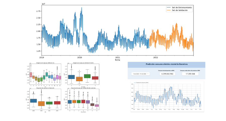
Transport
Sport
Culture and leisure
1. Introduction
Visualizations are graphical representations of data that allow the information linked to them to be communicated in a simple and effective way. The visualization possibilities are very wide, from basic representations, such as line, bar or sector graphs, to visualizations configured on interactive dashboards.
In this "Step-by-Step Visualizations" section we are regularly presenting practical exercises of open data visualizations available in datos.gob.es or other similar catalogs. They address and describe in a simple way the stages necessary to obtain the data, perform the transformations and analyses that are relevant to, finally, enable the creation of interactive visualizations that allow us to obtain final conclusions as a summary of said information. In each of these practical exercises, simple and well-documented code developments are used, as well as tools that are free to use. All generated material is available for reuse in the GitHub Data Lab repository.
Then, and as a complement to the explanation that you will find below, you can access the code that we will use in the exercise and that we will explain and develop in the following sections of this post.
Access the data lab repository on Github.
Run the data pre-processing code on top of Google Colab.
Back to top
2. Objetive
The main objective of this exercise is to show how to perform a network or graph analysis based on open data on rental bicycle trips in the city of Madrid. To do this, we will perform a preprocessing of the data in order to obtain the tables that we will use next in the visualization generating tool, with which we will create the visualizations of the graph.
Network analysis are methods and tools for the study and interpretation of the relationships and connections between entities or interconnected nodes of a network, these entities being persons, sites, products, or organizations, among others. Network analysis seeks to discover patterns, identify communities, analyze influence, and determine the importance of nodes within the network. This is achieved by using specific algorithms and techniques to extract meaningful insights from network data.
Once the data has been analyzed using this visualization, we can answer questions such as the following:
What is the network station with the highest inbound and outbound traffic?
What are the most common interstation routes?
What is the average number of connections between stations for each of them?
What are the most interconnected stations within the network?
Back to top
3. Resources
3.1. Datasets
The open datasets used contain information on loan bike trips made in the city of Madrid. The information they provide is about the station of origin and destination, the time of the journey, the duration of the journey, the identifier of the bicycle, ...
These open datasets are published by the Madrid City Council, through files that collect the records on a monthly basis.
Monthly series static data BICIMAD
These datasets are also available for download from the following Github repository.
3.2. Tools
To carry out the data preprocessing tasks, the Python programming language written on a Jupyter Notebook hosted in the Google Colab cloud service has been used.
"Google Colab" or, also called Google Colaboratory, is a cloud service from Google Research that allows you to program, execute and share code written in Python or R on a Jupyter Notebook from your browser, so it does not require configuration. This service is free of charge.
For the creation of the interactive visualization, the Gephi tool has been used.
"Gephi" is a network visualization and analysis tool. It allows you to represent and explore relationships between elements, such as nodes and links, in order to understand the structure and patterns of the network. The program requires download and is free.
If you want to know more about tools that can help you in the treatment and visualization of data, you can use the report "Data processing and visualization tools".
Back to top
4. Data processing or preparation
The processes that we describe below you will find them commented in the Notebook that you can also run from Google Colab.
Due to the high volume of trips recorded in the datasets, we defined the following starting points when analysing them:
We will analyse the time of day with the highest travel traffic
We will analyse the stations with a higher volume of trips
Before launching to analyse and build an effective visualization, we must carry out a prior treatment of the data, paying special attention to its obtaining and the validation of its content, making sure that they are in the appropriate and consistent format for processing and that they do not contain errors.
As a first step of the process, it is necessary to perform an exploratory analysis of the data (EDA), in order to properly interpret the starting data, detect anomalies, missing data or errors that could affect the quality of subsequent processes and results. If you want to know more about this process you can resort to the Practical Guide of Introduction to Exploratory Data Analysis
The next step is to generate the pre-processed data table that we will use to feed the network analysis tool (Gephi) that will visually help us understand the information. To do this, we will modify, filter and join the data according to our needs.
The steps followed in this data preprocessing, explained in this Google Colab Notebook, are as follows:
Installation of libraries and loading of datasets
Exploratory Data Analysis (EDA)
Generating pre-processed tables
You will be able to reproduce this analysis with the source code that is available in our GitHub account. The way to provide the code is through a document made on a Jupyter Notebook that, once loaded into the development environment, you can easily run or modify.
Due to the informative nature of this post and to favour the understanding of non-specialized readers, the code is not intended to be the most efficient but to facilitate its understanding, so you will possibly come up with many ways to optimize the proposed code to achieve similar purposes. We encourage you to do so!
Back to top
5. Network analysis
5.1. Definition of the network
The analysed network is formed by the trips between different bicycle stations in the city of Madrid, having as main information of each of the registered trips the station of origin (called "source") and the destination station (called "target").
The network consists of 253 nodes (stations) and 3012 edges (interactions between stations). It is a directed graph, because the interactions are bidirectional and weighted, because each edge between the nodes has an associated numerical value called "weight" which in this case corresponds to the number of trips made between both stations.
5.2. Loading the pre-processed table in to Gephi
Using the "import spreadsheet" option on the file tab, we import the previously pre-processed data table in CSV format. Gephi will detect what type of data is being loaded, so we will use the default predefined parameters.
Figure 1. Uploading data to Gephi
5.3. Network display options
5.3.1 Distribution window
First, we apply in the distribution window, the Force Atlas 2 algorithm. This algorithm uses the technique of node repulsion depending on the degree of connection in such a way that the sparsely connected nodes are separated from those with a greater force of attraction to each other.
To prevent the related components from being out of the main view, we set the value of the parameter "Severity in Tuning" to a value of 10 and to avoid that the nodes are piled up, we check the option "Dissuade Hubs" and "Avoid overlap".
Figure 2. Distribution window - Force Atlas 2 overlap
Dentro de la ventana de distribución, también aplicamos el algoritmo de Expansión con la finalidad de que los nodos no se encuentren tan juntos entre sí mismos.
Figure 3. Distribution window - Expansion algorithm
5.3.2 Appearance window
Next, in the appearance window, we modify the nodes and their labels so that their size is not equal but depends on the value of the degree of each node (nodes with a higher degree, larger visual size). We will also modify the colour of the nodes so that the larger ones are a more striking colour than the smaller ones. In the same appearance window we modify the edges, in this case we have opted for a unitary colour for all of them, since by default the size is according to the weight of each of them.
A higher degree in one of the nodes implies a greater number of stations connected to that node, while a greater weight of the edges implies a greater number of trips for each connection.
Figure 4. Appearance window
5.3.3 Graph window
Finally, in the lower area of the interface of the graph window, we have several options such as activating / deactivating the button to show the labels of the different nodes, adapting the size of the edges in order to make the visualization cleaner, modify the font of the labels, ...
Figure 5. Options graph window
Next, we can see the visualization of the graph that represents the network once the visualization options mentioned in the previous points have been applied.
Figure 6. Graph display
Activating the option to display labels and placing the cursor on one of the nodes, the links that correspond to the node and the rest of the nodes that are linked to the chosen one through these links will be displayed.
Next, we can visualize the nodes and links related to the bicycle station "Fernando el Católico". In the visualization, the nodes that have a greater number of connections are easily distinguished, since they appear with a larger size and more striking colours, such as "Plaza de la Cebada" or "Quevedo".
Figure 7. Graph display for station "Fernando el Católico"
5.4 Main network measures
Together with the visualization of the graph, the following measurements provide us with the main information of the analysed network. These averages, which are the usual metrics when performing network analytics, can be calculated in the statistics window.
Figure 8. Statistics window
Nodes (N): are the different individual elements that make up a network, representing different entities. In this case the different bicycle stations. Its value on the network is 243
Links (L): are the connections that exist between the nodes of a network. Links represent the relationships or interactions between the individual elements (nodes) that make up the network. Its value in the network is 3014
Maximum number of links (Lmax): is the maximum possible number of links in the network. It is calculated by the following formula Lmax= N(N-1)/2. Its value on the network is 31878
Average grade (k): is a statistical measure to quantify the average connectivity of network nodes. It is calculated by averaging the degrees of all nodes in the network. Its value in the network is 23.8
Network density (d): indicates the proportion of connections between network nodes to the total number of possible connections. Its value in the network is 0.047
Diámetro (dmax ): is the longest graph distance between any two nodes of the res, i.e., how far away the 2 nodes are farther apart. Its value on the network is 7
Mean distance (d):is the average mean graph distance between the nodes of the network. Its value on the network is 2.68
Mean clustering coefficient (C): Indicates how nodes are embedded between their neighbouring nodes. The average value gives a general indication of the grouping in the network. Its value in the network is 0.208
Related component: A group of nodes that are directly or indirectly connected to each other but are not connected to nodes outside that group. Its value on the network is 24
5.5 Interpretation of results
The probability of degrees roughly follows a long-tail distribution, where we can observe that there are a few stations that interact with a large number of them while most interact with a low number of stations.
The average grade is 23.8 which indicates that each station interacts on average with about 24 other stations (input and output).
In the following graph we can see that, although we have nodes with degrees considered as high (80, 90, 100, ...), it is observed that 25% of the nodes have degrees equal to or less than 8, while 75% of the nodes have degrees less than or equal to 32.
Figure 9. Grade Allocation Chart
The previous graph can be broken down into the following two corresponding to the average degree of input and output (since the network is directional). We see that both have similar long-tail distributions, their mean degree being the same of 11.9
Its main difference is that the graph corresponding to the average degree of input has a median of 7 while the output is 9, which means that there is a majority of nodes with lower degrees in the input than the output.
Figure 10. Graphs distribution of degrees of input and output
The value of the average grade with weights is 346.07 which indicates the average of total trips in and out of each station.
Figure 11. Graph distribution of degrees with weights
The network density of 0.047 is considered a low density indicating that the network is dispersed, that is, it contains few interactions between different stations in relation to the possible ones. This is considered logical because connections between stations will be limited to certain areas due to the difficulty of reaching stations that are located at long distances.
The average clustering coefficient is 0.208 meaning that the interaction of two stations with a third does not necessarily imply interaction with each other, that is, it does not necessarily imply transitivity, so the probability of interconnection of these two stations through the intervention of a third is low.
Finally, the network has 24 related components, of which 2 are weak related components and 22 are strong related components.
5.6 Centrality analysis
A centrality analysis refers to the assessment of the importance of nodes in a network using different measures. Centrality is a fundamental concept in network analysis and is used to identify key or influential nodes within a network. To perform this task, you start from the metrics calculated in the statistics window.
The degree centrality measure indicates that the higher the degree of a node, the more important it is. The five stations with the highest values are: 1º Plaza de la Cebada, 2º Plaza de Lavapiés, 3º Fernando el Católico, 4º Quevedo, 5º Segovia 45.
Figure 12. Graph visualization degree centrality
The closeness centrality indicates that the higher the proximity value of a node, the more central it is, since it can reach any other node in the network with the least possible effort. The five stations with the highest values are: 1º Fernando el Católico 2º General Pardiñas, 3º Plaza de la Cebada, 4º Plaza de Lavapiés, 5º Puerta de Madrid.
Figure 13. Measured closeness centrality distribution
Figure 14. Graphic visualization closeness centrality
The measure of betweenness centrality indicates that the greater the intermediation measure of a node, the more important it is since it is present in more interaction paths between nodes than the rest of the nodes in the network. The five stations with the highest values are: 1º Fernando el Católico, 2º Plaza de Lavapiés, 3º Plaza de la Cebada, 4º Puerta de Madrid, 5º Quevedo.
Figure 15. Measured betweenness centrality distribution
FIgure 16. Graphic visualization betweenness centrality
With the Gephi tool you can calculate a large number of metrics and parameters that are not reflected in this study, such as the eigenvector measure or centrality distribution "eigenvector".
5.7 Filters
Through the filtering window, we can select certain parameters that simplify the visualizations in order to show relevant information of network analysis in a clearer way visually.
Figure 17. Filtering windows
Next, we will show several filtered performed:
Range (grade) filtering, which shows nodes with a rank greater than 50, assuming 13.44% (34 nodes) and 15.41% (464 edges).
Figure 18. Graph display filtered range (degree)
Edge filtering (edge weight), showing edges weighing more than 100, assuming 0.7% (20 edges).
Figure 19. Visualization graph edge filtering (weight)
Within the filters window, there are many other filtering options on attributes, ranges, partition sizes, edges, ... with which you can try to make new visualizations to extract information from the graph. If you want to know more about the use of Gephi, you can consult the following courses and trainings about the tool.
Back to top
6. Conclusions of the exercice
Once the exercise is done, we can appreciate the following conclusions:
The three stations most interconnected with other stations are Plaza de la Cebada (133), Plaza de Lavapiés (126) and Fernando el Católico (114).
The station that has the highest number of input connections is Plaza de la Cebada (78), while the one with the highest number of exit connections is Plaza de Lavapiés with the same number as Fernando el Católico (57).
The three stations with the highest number of total trips are Plaza de la Cebada (4524), Plaza de Lavapiés (4237) and Fernando el Católico (3526).
There are 20 routes with more than 100 trips. Being the 3 routes with a greater number of them: Puerta de Toledo – Plaza Conde Suchil (141), Quintana Fuente del Berro – Quintana (137), Camino Vinateros – Miguel Moya (134).
Taking into account the number of connections between stations and trips, the most important stations within the network are: Plaza la Cebada, Plaza de Lavapiés and Fernando el Católico.
We hope that this step-by-step visualization has been useful for learning some very common techniques in the treatment and representation of open data. We will be back to show you further reuses. See you soon!
Back to top
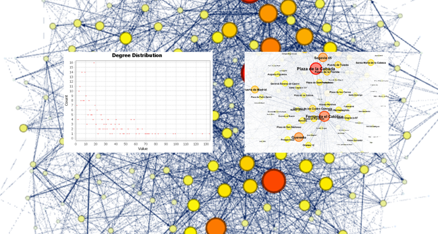
Commerce
Science and technology
1. Introduction
Visualizations are graphical representations of data that allow the information linked to them to be communicated in a simple and effective way. The visualization possibilities are very wide, from basic representations, such as line, bar or sector graphs, to visualizations configured on interactive dashboards.
In this "Step-by-Step Visualizations" section we are regularly presenting practical exercises of open data visualizations available in datos.gob.es or other similar catalogs. They address and describe in a simple way the stages necessary to obtain the data, perform the transformations and analyses that are relevant to, finally, enable the creation of interactive visualizations that allow us to obtain final conclusions as a summary of said information. In each of these practical exercises, simple and well-documented code developments are used, as well as tools that are free to use. All generated material is available for reuse in the GitHub Data Lab repository.
Then, as a complement to the explanation that you will find below, you can access the code that we will use in the exercise and that we will explain and develop in the following sections of this post.
Access the data lab repository on Github.
Run the data pre-processing code on top of Google Colab.
2. Objetive
The main objective of this exercise is to show how to generate an interactive dashboard that, based on open data, shows us relevant information on the food consumption of Spanish households based on open data. To do this, we will pre-process the open data to obtain the tables that we will use in the visualization generating tool to create the interactive dashboard.
Dashboards are tools that allow you to present information in a visual and easily understandable way. Also known by the term "dashboards", they are used to monitor, analyze and communicate data and indicators. Your content typically includes charts, tables, indicators, maps, and other visuals that represent relevant data and metrics. These visualizations help users quickly understand a situation, identify trends, spot patterns, and make informed decisions.
Once the data has been analyzed, through this visualization we will be able to answer questions such as those posed below:
What is the trend in recent years regarding spending and per capita consumption in the different foods that make up the basic basket?
What foods are the most and least consumed in recent years?
In which Autonomous Communities is there a greater expenditure and consumption in food?
Has the increase in the cost of certain foods in recent years meant a reduction in their consumption?
These, and many other questions can be solved through the dashboard that will show information in an orderly and easy to interpret way.
Back to top
3. Resources
3.1. Datasets
The open datasets used in this exercise contain different information on per capita consumption and per capita expenditure of the main food groups broken down by Autonomous Community. The open datasets used, belonging to the Ministry of Agriculture, Fisheries and Food (MAPA), are provided in annual series (we will use the annual series from 2010 to 2021)
Annual series data on household food consumption
These datasets are also available for download from the following Github repository.
Annual series data on hosehold food consumption
These datasets are also available for download from the following Github repository.
Back to top
3.2. Tools
To carry out the data preprocessing tasks, the Python programming language written on a Jupyter Notebook hosted in the Google Colab cloud service has been used.
"Google Colab" or, also called Google Colaboratory, is a cloud service from Google Research that allows you to program, execute and share code written in Python or R on a Jupyter Notebook from your browser, so it does not require configuration. This service is free of charge.
For the creation of the dashboard, the Looker Studio tool has been used.
"Looker Studio" formerly known as Google Data Studio, is an online tool that allows you to create interactive dashboards that can be inserted into websites or exported as files. This tool is simple to use and allows multiple customization options.
If you want to know more about tools that can help you in the treatment and visualization of data, you can use the report "Data processing and visualization tools".
Back to top
4. Processing or preparation of data
The processes that we describe below you will find commented in the following Notebook that you can run from Google Colab.
Before embarking on building an effective visualization, we must carry out a prior treatment of the data, paying special attention to its obtaining and the validation of its content, making sure that it is in the appropriate and consistent format for processing and that it does not contain errors.
As a first step of the process, once the initial data sets are loaded, it is necessary to perform an exploratory data analysis (EDA) to properly interpret the starting data, detect anomalies, missing data or errors that could affect the quality of subsequent processes and results. If you want to know more about this process, you can resort to the Practical Guide of Introduction to Exploratory Data Analysis.
The next step is to generate the pre-processed data table that we will use to feed the visualization tool (Looker Studio). To do this, we will modify, filter and join the data according to our needs.
The steps followed in this data preprocessing, explained in the following Google Colab Notebook, are as follows:
Installation of libraries and loading of datasets
Exploratory Data Analysis (EDA)
Generating preprocessed tables
You will be able to reproduce this analysis with the source code that is available in our GitHub account. The way to provide the code is through a document made on a Jupyter Notebook that once loaded into the development environment you can run or modify easily. Due to the informative nature of this post and to favor the understanding of non-specialized readers, the code is not intended to be the most efficient, but to facilitate its understanding so you will possibly come up with many ways to optimize the proposed code to achieve similar purposes. We encourage you to do so!
Back to top
5. Displaying the interactive dashboard
Once we have done the preprocessing of the data, we go with the generation of the dashboard. A scorecard is a visual tool that provides a summary view of key data and metrics. It is useful for monitoring, decision-making and effective communication, by providing a clear and concise view of relevant information.
For the realization of the interactive visualizations that make up the dashboard, the Looker Studio tool has been used. Being an online tool, it is not necessary to have software installed to interact or generate any visualization, but it is necessary that the data table that we provide is properly structured, which is why we have carried out the previous steps related to the preprocessing of the data. If you want to know more about how to use Looker Studio, in the following link you can access training on the use of the tool.
Below is the dashboard, which can be opened in a new tab in the following link. In the following sections we will break down each of the components that make it up.
5.1. Filters
Filters in a dashboard are selection options that allow you to visualize and analyze specific data by applying various filtering criteria to the datasets presented in the dashboard. They help you focus on relevant information and get a more accurate view of your data.
Figure 1. Filters dashboard
The filters included in the generated dashboard allow you to choose the type of analysis to be displayed, the territory or Autonomous Community, the category of food and the years of the sample.
It also incorporates various buttons to facilitate the deletion of the chosen filters, download the dashboard as a report in PDF format and access the raw data with which this dashboard has been prepared.
5.2. Interactive visualizations
The dashboard is composed of various types of interactive visualizations, which are graphical representations of data that allow users to actively explore and manipulate information.
Unlike static visualizations, interactive visualizations provide the ability to interact with data, allowing users to perform different and interesting actions such as clicking on elements, dragging them, zooming or reducing focus, filtering data, changing parameters and viewing results in real time.
This interaction is especially useful when working with large and complex data sets, as it makes it easier for users to examine different aspects of the data as well as discover patterns, trends and relationships in a more intuitive way.
To define each type of visualization, we have based ourselves on the data visualization guide for local entities presented by the NETWORK of Local Entities for Transparency and Citizen Participation of the FEMP.
5.2.1 Data tables
Data tables allow the presentation of a large amount of data in an organized and clear way, with a high space/information performance.
However, they can make it difficult to present patterns or interpretations with respect to other visual objects of a more graphic nature.
Figure 3. Dashboard data table
5.2.2 Map of chloropetas
t is a map in which numerical data are shown by territories marking with intensity of different colours the different areas. For its elaboration it requires a measure or numerical data, a categorical data for the territory and a geographical data to delimit the area of each territory.
Figure 3. Dashboard Chloropeta Map
5.2.3 Pie chart
It is a graph that shows the data from polar axes in which the angle of each sector marks the proportion of a category with respect to the total. Its functionality is to show the different proportions of each category with respect to a total using pie charts.
Figure 4. Dashboard pie chart
5.2.4 Line chart
It is a graph that shows the relationship between two or more measurements of a series of values on two Cartesian axes, reflecting on the X axis a temporal dimension, and a numerical measure on the Y axis. These charts are ideal for representing time data series with a large number of data points or observations.
Figure 5. Dashboard line chart
5.2.5 Bar chart
It is a graph of the most used for the clarity and simplicity of preparation. It makes it easier to read values from the ratio of the length of the bars. The chart displays the data using an axis that represents the quantitative values and another that includes the qualitative data of the categories or time.
Figure 6. Dashboard bar chart
5.2.6 Hierarchy chart
It is a graph formed by different rectangles that represent categories, and that allows hierarchical groupings of the sectors of each category. The dimension of each rectangle and its placement varies depending on the value of the measurement of each of the categories shown with respect to the total value of the sample.
Figure 7. Dashboard Hierarchy chart
Back to top
6. Conclusions
Dashboards are one of the most powerful mechanisms for exploiting and analyzing the meaning of data. It should be noted the importance they offer us when it comes to monitoring, analyzing and communicating data and indicators in a clear, simple and effective way.
As a result, we have been able to answer the questions originally posed:
The trend in per capita consumption has been declining since 2013, when it peaked, with a small rebound in 2020 and 2021.
The trend of per capita expenditure has remained stable since 2011 until in 2020 it has suffered a rise of 17.7%, going from being the average annual expenditure of 1052 euros to 1239 euros, producing a slight decrease of 4.4% from the data of 2020 to those of 2021.
The three most consumed foods during all the years analyzed are: fresh fruits, liquid milk and meat (values in kgs)
The Autonomous Communities where per capita spending is highest are the Basque Country, Catalonia and Asturias, while Castilla la Mancha, Andalusia and Extremadura have the lowest spending.
The Autonomous Communities where a higher per capita consumption occurs are Castilla y León, Asturias and the Basque Country, while in those with the lowest are Extremadura, the Canary Islands and Andalusia.
We have also been able to observe certain interesting patterns, such as a 17.33% increase in alcohol consumption (beers, wine and spirits) in the years 2019 and 2020.
You can use the different filters to find out and look for more trends or patterns in the data based on your interests and concerns.
We hope that this step-by-step visualization has been useful for learning some very common techniques in the treatment and representation of open data. We will be back to show you new reuses. See you soon!
Back to top
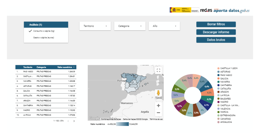
Environment
Science and technology
1. Introduction
Visualizations are graphical representations of data that allow the information linked to them to be communicated in a simple and effective way. The visualization possibilities are very wide, from basic representations, such as a line chart, bars or sectors, to visualizations configured on dashboards or interactive dashboards.
In this "Step-by-Step Visualizations" section we are regularly presenting practical exercises of open data visualizations available on datos.gob.es or similar catalogs. They address and describe in a simple way the stages necessary to obtain the data, perform the transformations and analysis that are relevant to and finally, the creation of interactive visualizations; from which we can extract information summarized in final conclusions. In each of these practical exercises, simple and well-documented code developments are used, as well as free to use tools. All generated material is available for reuse in GitHub's Data Lab repository.
Run the data pre-processing code on top of Google Colab.
Below, you can access the material that we will use in the exercise and that we will explain and develop in the following sections of this post.
Access the data lab repository on Github.
Run the data pre-processing code on top of Google Colab.
Back to top
2. Objective
The main objective of this exercise is to make an analysis of the meteorological data collected in several stations during the last years. To perform this analysis, we will use different visualizations generated by the "ggplot2" library of the programming language "R".
Of all the Spanish weather stations, we have decided to analyze two of them, one in the coldest province of the country (Burgos) and another in the warmest province of the country (Córdoba), according to data from the AEMET. Patterns and trends in the different records between 1990 and 2020 will be sought to understand the meteorological evolution suffered in this period of time.
Once the data has been analyzed, we can answer questions such as those shown below:
What is the trend in the evolution of temperatures in recent years?
What is the trend in the evolution of rainfall in recent years?
Which weather station (Burgos or Córdoba) presents a greater variation of climatological data in recent years?
What degree of correlation is there between the different climatological variables recorded?
These, and many other questions can be solved by using tools such as ggplot2 that facilitate the interpretation of data through interactive visualizations.
Back to top
3. Resources
3.1. Datasets
The datasets contain different meteorological information of interest for the two stations in question broken down by year. Within the AEMET download center, we can download them, upon request of the API key, in the section "monthly / annual climatologies". From the existing weather stations, we have selected two of which we will obtain the data: Burgos airport (2331) and Córdoba airport (5402)
It should be noted that, along with the datasets, we can also download their metadata, which are of special importance when identifying the different variables registered in the datasets.
These datasets are also available in the Github repository.
Back to top
3.2. Tools
To carry out the data preprocessing tasks, the R programming language written on a Jupyter Notebook hosted in the Google Colab cloud service has been used.
"Google Colab" or, also called Google Colaboratory, is a cloud service from Google Research that allows you to program, execute and share code written in Python or R on a Jupyter Notebook from your browser, so it does not require configuration. This service is free of charge.
For the creation of the visualizations, the ggplot2 library has been used.
"ggplot2" is a data visualization package for the R programming language. It focuses on the construction of graphics from layers of aesthetic, geometric and statistical elements. ggplot2 offers a wide range of high-quality statistical charts, including bar charts, line charts, scatter plots, box and whisker charts, and many others.
If you want to know more about tools that can help you in the treatment and visualization of data, you can use the report "Data processing and visualization tools".
Back to top
4. Data processing or preparation
The processes that we describe below you will find them commented in the Notebook that you can also run from Google Colab.
Before embarking on building an effective visualization, we must carry out a prior treatment of the data, paying special attention to obtaining them and validating their content, ensuring that they are in the appropriate and consistent format for processing and that they do not contain errors.
As a first step of the process, once the necessary libraries have been imported and the datasets loaded, it is necessary to perform an exploratory analysis of the data (EDA) in order to properly interpret the starting data, detect anomalies, missing data or errors that could affect the quality of the subsequent processes and results. If you want to know more about this process, you can resort to the Practical Guide of Introduction to Exploratory Data Analysis.
The next step is to generate the preprocessed data tables that we will use in the visualizations. To do this, we will filter the initial data sets and calculate the values that are necessary and of interest for the analysis carried out in this exercise.
Once the preprocessing is finished, we will obtain the data tables "datos_graficas_C" and "datos_graficas_B" which we will use in the next section of the Notebook to generate the visualizations.
The structure of the Notebook in which the steps previously described are carried out together with explanatory comments of each of them, is as follows:
Installation and loading of libraries.
Loading datasets
Exploratory Data Analysis (EDA)
Preparing the data tables
Views
Saving graphics
You will be able to reproduce this analysis, as the source code is available in our GitHub account. The way to provide the code is through a document made on a Jupyter Notebook that once loaded into the development environment you can run or modify easily. Due to the informative nature of this post and in order to favor the understanding of non-specialized readers, the code is not intended to be the most efficient but to facilitate its understanding so you will possibly come up with many ways to optimize the proposed code to achieve similar purposes. We encourage you to do so!
Back to top
5. Visualizations
Various types of visualizations and graphs have been made to extract information on the tables of preprocessed data and answer the initial questions posed in this exercise. As mentioned previously, the R "ggplot2" package has been used to perform the visualizations.
The "ggplot2" package is a data visualization library in the R programming language. It was developed by Hadley Wickham and is part of the "tidyverse" package toolkit. The "ggplot2" package is built around the concept of "graph grammar", which is a theoretical framework for building graphs by combining basic elements of data visualization such as layers, scales, legends, annotations, and themes. This allows you to create complex, custom data visualizations with cleaner, more structured code.
If you want to have a summary view of the possibilities of visualizations with ggplot2, see the following "cheatsheet". You can also get more detailed information in the following "user manual".
5.1. Line charts
Line charts are a graphical representation of data that uses points connected by lines to show the evolution of a variable in a continuous dimension, such as time. The values of the variable are represented on the vertical axis and the continuous dimension on the horizontal axis. Line charts are useful for visualizing trends, comparing evolutions, and detecting patterns.
Next, we can visualize several line graphs with the temporal evolution of the values of average, minimum and maximum temperatures of the two meteorological stations analyzed (Córdoba and Burgos). On these graphs, we have introduced trend lines to be able to observe their evolution in a visual and simple way.
To compare the evolutions, not only visually through the graphed trend lines, but also numerically, we obtain the slope coefficients of the trend line, that is, the change in the response variable (tm_ month, tm_min, tm_max) for each unit of change in the predictor variable (year).
Average temperature slope coefficient Córdoba: 0.036
Average temperature slope coefficient Burgos: 0.025
Coefficient of slope minimum temperature Córdoba: 0.020
Coefficient of slope minimum temperature Burgos: 0.020
Slope coefficient maximum temperature Córdoba: 0.051
Slope coefficient maximum temperature Burgos: 0.030
We can interpret that the higher this value, the more abrupt the average temperature rise in each observed period.
Finally, we have created a line graph for each weather station, in which we jointly visualize the evolution of average, minimum and maximum temperatures over the years.
The main conclusions obtained from the visualizations of this section are:
The average, minimum and maximum annual temperatures recorded in Córdoba and Burgos have an increasing trend.
The most significant increase is observed in the evolution of the maximum temperatures of Córdoba (slope coefficient = 0.051)
The slightest increase is observed in the evolution of the minimum temperatures, both in Córdoba and Burgos (slope coefficient = 0.020)
5.2. Bar charts
Bar charts are a graphical representation of data that uses rectangular bars to show the magnitude of a variable in different categories or groups. The height or length of the bars represents the amount or frequency of the variable, and the categories are represented on the horizontal axis. Bar charts are useful for comparing the magnitude of different categories and for visualizing differences between them.
We have generated two bar graphs with the data corresponding to the total accumulated precipitation per year for the different weather stations.
As in the previous section, we plot the trend line and calculate the slope coefficient.
Slope coefficient for accumulated rainfall Córdoba: -2.97
Slope coefficient for accumulated rainfall Burgos: -0.36
The main conclusions obtained from the visualizations of this section are:
The annual accumulated rainfall has a decreasing trend for both Córdoba and Burgos.
The downward trend is greater for Córdoba (coefficient = -2.97), being more moderate for Burgos (coefficient = -0.36)
5.3. Histograms
Histograms are a graphical representation of a frequency distribution of numeric data in a range of values. The horizontal axis represents the values of the data divided into intervals, called "bin", and the vertical axis represents the frequency or amount of data found in each "bin". Histograms are useful for identifying patterns in data, such as distribution, dispersion, symmetry, or bias.
We have generated two histograms with the distributions of the data corresponding to the total accumulated precipitation per year for the different meteorological stations, being the chosen intervals of 50 mm3.
The main conclusions obtained from the visualizations of this section are:
The records of annual accumulated precipitation in Burgos present a distribution close to a normal and symmetrical distribution.
The records of annual accumulated precipitation in Córdoba do not present a symmetrical distribution.
5.4. Box and whisker diagrams
Box and whisker diagrams are a graphical representation of the distribution of a set of numerical data. These graphs represent the median, interquartile range, and minimum and maximum values of the data. The chart box represents the interquartile range, that is, the range between the first and third quartiles of the data. Out-of-the-box points, called outliers, can indicate extreme values or anomalous data. Box plots are useful for comparing distributions and detecting extreme values in your data.
We have generated a graph with the box diagrams corresponding to the accumulated rainfall data from the weather stations.
To understand the graph, the following points should be highlighted:
The boundaries of the box indicate the first and third quartiles (Q1 and Q3), which leave below each, 25% and 75% of the data respectively.
The horizontal line inside the box is the median (equivalent to the second quartile Q2), which leaves half of the data below.
The whisker limits are the extreme values, that is, the minimum value and the maximum value of the data series.
The points outside the whiskers are the outliers.
The main conclusions obtained from the visualization of this section are:
Both distributions present 3 extreme values, being significant those of Córdoba with values greater than 1000 mm3.
The records of Córdoba have a greater variability than those of Burgos, which are more stable
5.5. Pie charts
A pie chart is a type of pie chart that represents proportions or percentages of a whole. It consists of several sections or sectors, where each sector represents a proportion of the whole set. The size of the sector is determined based on the proportion it represents, and is expressed in the form of an angle or percentage. It is a useful tool for visualizing the relative distribution of the different parts of a set and facilitates the visual comparison of the proportions between the different groups.
We have generated two graphs of (polar) sectors. The first of them with the number of days that the values exceed 30º in Córdoba and the second of them with the number of days that the values fall below 0º in Burgos.
For the realization of these graphs, we have grouped the sum of the number of days described above into six groups, corresponding to periods of 5 years from 1990 to 2020.
The main conclusions obtained from the visualizations of this section are:
There is an increase of 31.9% in the total number of annual days with temperatures above 30º in Córdoba for the period between 2015-2020 compared to the period 1990-1995.
There is an increase of 33.5% in the total number of annual days with temperatures above 30º in Burgos for the period between 2015-2020 compared to the period 1990-1995.
5.6. Scatter plots
Scatter plots are a data visualization tool that represent the relationship between two numerical variables by locating points on a Cartesian plane. Each dot represents a pair of values of the two variables and its position on the graph indicates how they relate to each other. Scatter plots are commonly used to identify patterns and trends in data, as well as to detect any possible correlation between variables. These charts can also help identify outliers or data that doesn't fit the overall trend.
We have generated two scattering plots in which the values of maximum average temperatures and minimum averages are compared, looking for correlation trends between them for the values of each weather station.
To analyze the correlations, not only visually through graphs, but also numerically, we obtain Pearson's correlation coefficients. This coefficient is a statistical measure that indicates the degree of linear association between two quantitative variables. It is used to assess whether there is a positive linear relationship (both variables increase or decrease simultaneously at a constant rate), negative (the values of both variables vary oppositely) or null (no relationship) between two variables and the strength of such a relationship, the closer to +1, the higher their association.
Pearson coefficient (Average temperature max VS min) Córdoba: 0.15
Pearson coefficient (Average temperature max VS min) Burgos: 0.61
In the image we observe that while in Córdoba a greater dispersion is appreciated, in Burgos a greater correlation is observed.
Next, we will modify the previous scatter plots so that they provide us with more information visually. To do this, we divide the space by colored sectors (red with higher temperature values / blue lower temperature values) and show in the different bubbles the label with the corresponding year. It should be noted that the color change limits of the quadrants correspond to the average values of each of the variables.
The main conclusions obtained from the visualizations of this section are:
There is a positive linear relationship between the average maximum and minimum temperature in both Córdoba and Burgos, this correlation being greater in the Burgos data.
The years with the highest values of maximum and minimum temperatures in Burgos are (2003, 2006 and 2020)
The years with the highest values of maximum and minimum temperatures in Córdoba are (1995, 2006 and 2020)
5.7. Correlation matrix
The correlation matrix is a table that shows the correlations between all variables in a dataset. It is a square matrix that shows the correlation between each pair of variables on a scale ranging from -1 to 1. A value of -1 indicates a perfect negative correlation, a value of 0 indicates no correlation, and a value of 1 indicates a perfect positive correlation. The correlation matrix is commonly used to identify patterns and relationships between variables in a dataset, which can help to better understand the factors that influence a phenomenon or outcome.
We have generated two heat maps with the correlation matrix data for both weather stations.
The main conclusions obtained from the visualizations of this section are:
There is a strong negative correlation (-0.42) for Córdoba and (-0.45) for Burgos between the number of annual days with temperatures above 30º and accumulated rainfall. This means that as the number of days with temperatures above 30º increases, precipitation decreases significantly.
6. Conclusions of the exercise
Data visualization is one of the most powerful mechanisms for exploiting and analyzing the implicit meaning of data. As we have seen in this exercise, "ggplot2" is a powerful library capable of representing a wide variety of graphics with a high degree of customization that allows you to adjust numerous characteristics of each graph.
After analyzing the previous visualizations, we can conclude that both for the weather station of Burgos, as well as that of Córdoba, temperatures (minimum, average, maximum) have suffered a considerable increase, days with extreme heat (temperature > 30º) have also suffered and rainfall has decreased in the period of time analyzed, from 1990 to 2020.
We hope that this step-by-step visualization has been useful for learning some very common techniques in the treatment, representation and interpretation of open data. We will be back to show you new reuses. See you soon!