28 data exercises found

Science and technology
Introduction
The National Institute of Statistics (INE) provides citizens with geographic data of social interest distributed by census sections. The use of these territorial units is, however, uncommon outside the statistical field. On the other hand, it is common to associate geographic data and variables with postal codes, since citizens are more familiar with their location and extent in their respective municipalities or provinces. For this reason, several public organizations, as well as private initiatives, collect and publish data associated with postal codes based on this familiarity.
This exercise details a method to establish a correspondence and extrapolate the associated data from census sections to their corresponding postal codes. This relationship is not direct, since the boundaries of both territorial units do not exactly coincide; that is, within the area of a postal code we find several complete census sections, and likewise, the same postal code can extend over more than one postal code. The lack of full match between both concepts requires methods to be able to extrapolate the information contained from one to the other with rigor and precision.
For this exercise, we will use INE data on average net income per person, originally available by census section, to estimate its value by postal code. Subsequently, these results will be related to the distribution of sports facilities in the province of Seville, distinguishing between Seville city and the rest of the province.
Based on this data, an exploratory analysis will be carried out aimed at identifying possible patterns related to:
The differences in the distribution of facilities by rent between Seville city and the rest of the province of Seville.
Differences in the distribution of basketball courts and gyms by rental.
The results will serve to identify territorial differences and formulate hypotheses that may help guide subsequent analyses of the coverage and distribution of these facilities, without establishing causal relationships between income level and their location.
Open geographic and statistical data from various public bodies will be used for them.
Definitions
In this exercise, we will cover the concepts of census section and postal code, which are defined below to facilitate understanding of the analysis.
Census section: it is a territorial unit used for collecting statistical information and organizing electoral processes. Generally, each census section has a size between 500 and 2000 inhabitants to facilitate the operation of pollsters and voters. Its boundaries are defined by easily identifiable elements, such as rivers or streets, which allows for clear geographic identification.
Figure 1: Census sections corresponding to the province of Seville and Seville city. Source: own elaboration based on data from the National Institute of Statistics (INE)
Postal code: this is a code that in Spain consists of five digits assigned to a specific area or geographic region to speed up the sorting, access, and delivery of postal shipments. The first two digits indicate the province in alphabetical order. The last three digits identify the municipality, postal zone, or delivery route.
Figure 2: Postal codes corresponding to the province of Seville. Source: own elaboration based on data from the National Geographic Institute (IGN).
Based on the previous definitions, Figure 3 shows the overlap of census sections and postal codes of Seville city and its surroundings, as well as the intersection zones that will be used later in the analysis.
Figure 3: Overlap of census sections and postal codes of Seville city and its surroundings. Source: own elaboration based on data from INE and IGN.
Datasets
Once the geographic units within which the study is framed are defined, we use open data from public organizations to carry out the exercise. Specifically, we will use the following data sets:
Geometry of the census tracts of the National Institute of Statistics for the year 2023..
Geometry of the postal codes in the province of Seville .
List of road sections of census sections by postal code,from the National Institute of Statistics.
Average net income per person by census section from the National Institute of Statistics.
Census of sport facilities in Andalusia, which includes information about their location - location by street, municipality, province, and postal code - and type of sports facility.
Development process
In this section, we will detail the steps to follow to associate the average net income per person of each census section with the location of sports facilities in Seville city and the rest of the province. Once we obtain the distribution of facilities by income, the analysis is deepened to study the differences between the two territories, as well as between the types of facilities depending on the sport practiced.
The analysis was developed in Python. Additionally, the Kepler.gl cartographic visualization software was used, which is easy and intuitive to use, and was already described in the execise on data visualization on earthquakes in the island of La Palma.
The Python code as well as the datasets already downloaded for processing are available in the Github repository:
Access the Github repository
The Google Colab notebook with all the commands needed to run the analysis in Python can be found at:
Access the GoogleColab notebook
1. Weight of census tracts in each postal code
The first step in this exercise is to calculate the weight of each census section in each postal code. To do this, we read the input file containing the road sections of each census section. In the reading, we first identify the codes for: province, municipality, district, and section
With these codes, we create the census section code by concatenation. A first example is found in the first entry of the file "List of road sections," where we observe the following values for the previously described fields: province: 41; municipality: 001; district: 01; section: 001
The resulting census section for that section of road is 4100101001, obtained by concatenating those fields according to the described order.
Once the census section is defined, we calculate how many times the unique combination census section and postal code appears. Next, we calculate the total number of road sections in each census section and, finally, the proportion of those sections corresponding to each postal code. In this way, we obtain the so-called weight matrix, where each combination of census section and postal code has an associated fraction or weight. Most census sections have a weight of 1 or fraction unit, which means that all their road sections are associated with a single postal code. Other census sections are divided into two or more postal codes.
In total, out of the 1,595 census tracts in the province of Seville, we obtain 1,207 census tracts whose tracts are entirely associated with a postal code, while 388 have tracts associated with more than one postal code.
Figure 4 shows the geographical distribution of census sections according to the weight of their road sections in postal codes, both in the province of Seville and in Seville city. It is observed that sections whose sections are associated with more than one postal code are located in both urban and rural areas.
Figure 4: Census sections of the province of Seville and Seville city according to the weight of their road sections in postal codes. Source: own elaboration.
Focusing on the city of Seville, it is clear how, once again, the disparity of pesos is distributed throughout the city's geography. The results highlight the need to apply these weights and to estimate the values corresponding to each postal code based on data available by census section.
2. Income association to each postal code
The next step in this exercise is to associate the average net income per person values with postal codes.
Below we can see how the INE data are structured regarding the average net income per person and the assigned census section. Specifically, Table 1 shows two census sections, belonging to different census districts of the municipality of Aguadulce, with different income values. Both sections are associated with a single postal code, and therefore, the estimated income for that postal code will result from the weighted average of the income values of the associated census sections, using the weights calculated in the previous section.
Table 1: Sample data on average net income per person and census section for the municipality of Aguadulce. Source: INE.
The result of weighting the contributions of the different census sections to estimate the average net income per person of a postal code can be seen in Table 2, following the previous example of the municipality of Aguadulce. The value obtained falls within the income values shown in Table 1.
Variable
Value
Municipality
41001
Postal code
41550
Averaged rent per person
10.539
Table 2: Estimate of the average net income per person for postal code 41550 corresponding to the Municipality with census code 41001. Source: own elaboration.
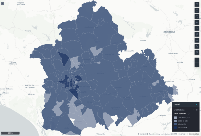
The geographical distribution of the estimated average income per person for each postal code of the province of Seville can be seen in Figure 5. It shows how the lowest incomes are located on the periphery of the province, while the highest incomes are located in urban centers, particularly in Seville city.
Figure 5: Distribution of the estimated average net income per person for each postal code of the province of Seville and Seville city. Source: own elaboration.
3. Association of sports facilities at the rental level
The next step is to establish the association of the location of sports facilities with the estimated income level for each postal code.
Table 3 shows the structure of the data set for sports facilities in Andalusia. It details the location of the facility, the municipality, the name of the road, and the postal code. It also includes the type of facility, determined by the sport practiced.
Variable
Value
IDA code
2
Facility name
PABELLON DEPORTIVO CUBIERTO
Province
Sevilla
Municipality
Castilblanco de los Arroyos
Street
CAMINO DEL TOLEDILLO
Postal code
41230
Type of facility
PISTA POLIDEPORTIVA
Table 3: Structure of the dataset of sports centers in Andalusia. Source: Junta de Andalucía.
Thanks to the correspondence obtained between estimated income values and postal codes in the previous step, we can expand the information associated with each sports facility by incorporating a new field: the estimated average net income per person for its postal code. Table 4 shows the new field included.
Variable
Value
IDA code
2
Facility name
PABELLON DEPORTIVO CUBIERTO
Province
Sevilla
Municipality
Castilblanco de los Arroyos
Street
CAMINO DEL TOLEDILLO
Postal code
41230
Type of facility
PISTA POLIDEPORTIVA
Rent per person
10.620
Table 4: Structure of the dataset of sports centers in Andalusia complemented by the estimated average net income per person. Source: own elaboration.
In this way, we have managed to relate the estimated average net income per person for each postal code with the sports facilities in Seville province or capital.
This result then allows us to develop a whole series of statistical analyses to identify possible patterns and describe the distribution of sports facilities, as presented in the following section.
4. Location of sports facilities relative to average income
By taking the average income per person both in the province of Seville and in Seville city, it is possible to identify how sports facilities are distributed relative to that average. In this way, we can observe whether facilities are located in postal codes with an estimated income lower or higher than the average of each territorial area.
At this point, we make a distinction between the province of Seville without capital and Seville as capital, as they are two very different environments. At the provincial level, we find a more dispersed population, postal codes covering a larger area, and a concentration of services in population centers.
On the other hand, in Seville city we generally find areas with smaller postal codes and a higher concentration of sports facilities outside the city center, commonly associated with sports such as football, gyms, padel courts, or swimming pools.
Figure 6 shows the number of sports facilities by average income per person estimated for their postal code in three areas: the province of Seville as a whole, the province without the capital, and the capital itself. In these three regions we observe:
Across the province, the highest concentration of facilities is found in postal codes with income values close to the provincial average, although the distribution is more frequent in some intervals slightly above it.
Compared to the province of Seville without the capital, the highest concentration of installations is also in postal codes with income values close to the average for this area. Likewise, a notable number of installations in postal codes is observed with an average net income per person below 5,000 euros per year.
In the case of Seville city, the distribution shows greater dispersion among the different income brackets. The facilities are distributed over a wider range of values, and there is not as pronounced a concentration in a single income bracket as in the rest of the province.
Figure 6: Number of sports facilities by estimated income per person for their postal code in the province of Seville, the province without capital, and Seville capital. The vertical lines indicate the estimated average income in each territorial area. Source: own elaboration
Considering the dispersion in income values, we see in Figure 7 how, despite sharing almost the same spectrum of possible incomes, at the provincial level the concentration is much greater around a low one around the average income, while in the case of Seville city sports facilities cover an interval almost twice as wide as in the province. This leads us to reflect on the homogenizing effect of cities, where a smaller space coexists with a broader income spectrum than in the province.
5. Distribution of sports facilities by type of sport
The last analysis addressed the variability associated with the type of sport practiced and, therefore, the type of sports facility. Different sports have different space needs and may be associated with different user profiles. In this preliminary analysis, we distinguish between two types of facilities, basketball courts and gyms, to perform the same calculation as in the previous section.
By filtering the data using the keywords "baloncesto" and "gimnasio" in the free text field corresponding to the sports area, we can generate a histogram for the case of Seville city and analyze the distribution of sports facilities in relation to the average income per person for each postal code. Figure 7 and Figure 8 show the results by sport, where we find:
In the case of basketball courts, the histogram distribution in Seville city shifts slightly towards income values below the average. In total, 67% of basketball courts are in postal codes with estimated average income per person below the average for Seville city.
Gyms, on the other hand, shift the histogram to the right compared to basketball courts, toward a balanced distribution according to income level. 55% of gyms are in postal codes whose estimated average income per person is below the city's average income.
a {
text-decoration: none;
color: #464feb;
}
tr th, tr td {
border: 1px solid #e6e6e6;
}
tr th {
background-color: #f5f5f5;
}
Figura 7: Distribution of basketball courts according to the estimated average net income per person for its postal code in Seville city. Source: own elaboration.
Figure 8: Distribution of basketball courts according to the estimated average net income per person for its postal code in Seville city. Source: own elaboration.
These results reveal differences in the territorial distribution of both types of facilities regarding the estimated income of the postal codes where they are located. However, additional variables would be necessary to analyze the causes that may explain these differences.
Lessons learned
Throughout this analysis exercise, we have learned to handle INE data by census sections, to estimate values originally available by census section by postal code, to apply this procedure to a real case linked to a data set from the Catalog, and to carry out a brief exploratory statistical analysis that allows us to identify patterns and formulate hypotheses for later analysis. Specifically, we have learned to:
Differentiate between census section and postal code, from its most basic definition to real examples of both units in a specific province.
Reading INE files with information grouped by census sections and detailed by provinces, municipalities, and districts, as well as creating the census section code.
Calculate the relative weight of each census section in different postal codes, delving into their complexity and taking into account the correspondence differences between both territorial units
Apply filters in Python to select data by postal code or specific text fields, such as the selected sports, thus focusing the analysis on specific cases.
Create visualizations in Python to perform basic statistical analysis, such as the histogram.
Use Kepler.gl to create maps easily and intuitively to accompany georeferenced data exercises.
Conclusions
This exercise has allowed us to become familiar with the concept of a census section, from accessing, reading, and manipulating the original INE files to a real application with data from the Junta de Andalucía.
Likewise, it has allowed us to verify how a simple and relatively short Python script is sufficient for reading and analyzing INE data, as well as for exploratory statistical analysis of that and other related datasets, demonstrating the potential of programming.
Finally, this exercise invites the formulation of a whole series of hypotheses about the distribution of public resources by income level, as well as reflection on how the city structures that distribution and with what criteria, which go beyond the focus of this simple exercise.
Next steps
From this exercise, the analysis could be expanded by incorporating new variables, such as the population of each postal code, ownership and capacity of the facilities, or their degree of utilization. This would allow calculating comparable indicators, such as the number of facilities per 10,000 inhabitants, and deepening the study of their territorial distribution. The same procedure could also be applied to other services and facilities, such as educational, health, or cultural centers.

Science and technology
Introduction
The celestial dance of the stars in the solar system offers unique and singular spectacles from time to time, such as the entire total eclipses that took place in the Iberian Peninsula this year, and that will happen in 2027 and 2028. During a total eclipse, the Moon comes between the Earth and the Sun, hiding the sun and casting a shadow on a part of the Earth's surface for a few minutes.
The total eclipse of August 12, 2026 began at around 8:30 p.m. (GMT+01:00), covering the penumbra from Galicia to the Balearic Islands throughout the hour and a half duration of the eclipse.
The National Center for Geographic Information (CNIG) has made available to the public datasets that offer a wide spectrum of astronomical information related to the eclipse that occurred over the Iberian Peninsula in 2026, as well as those that will happen over the next two years.
These datasets include information on the visibility of the terrain itself at the time of the eclipse, the duration of the eclipse at each point of the Spanish geography, the level of obscuration or elevation of the Sun at the maximum point of the eclipse, as well as the shadow cast by the Moon on its path in front of the Sun.
In this exercise we will access the data sets of the CNIG and open the .TIF and .GPKG files with all the information related to the eclipse, and specifically with everything related to the shadow areas, both in terms of visibility due to the effect of the relief on the peninsula, and with regard to the shadow area itself due to the total eclipse.
Once we have accessed the data, we will limit our analysis to a specific area on visibility by relief, we will cut the original data with the perimeter of a municipality, we will export the result in GeoJSON format and, making use of it, we will be able to create different types of maps with various useful and intuitive tools such as KeplerGL, GoogleEarth, Leaflet or D3.js.
Data for the exercise
The data available to carry out this exercise are accessible in the Catalog of open data of datos.gob.es, there are three files with relevant information to describe and characterize the eclipse. Specifically, we find:
Terrain shadows: File describing visibility by relief in a mesh of dots covering the Iberian Peninsula and the western part of North Africa.
Contour Lines: A file containing the duration, maximum dimming, and penumbra curves projected from the Moon onto the Earth.
Ephemeris: File that houses the eclipse ephemeris, such as elevation, azimuth, sunrise and sunset, as well as the beginning and end of the eclipse.
In this exercise we will focus on the first two, as they contain information on the shadow cast by both the relief and the Moon on the Iberian Peninsula.
In addition, we will also use the Data Catalogue to obtain the perimeter in SHP format of a municipality that allows us to analyse in detail the shadow by relief. In this way we will complete the access and reading of three different georeferenced data formats:
TIFF: A popular format for high-resolution graphic information that tolerates high degrees of lossless compression and is therefore very manageable. The acronym stands for Tagged Image File Format.
GPKG: An acronym for GeoPackage. This format is used in geographic information systems to store data in both radara and vector modes.
SHP: vector data format containing geometric locations, also widely used in geographic information systems. It contains exclusively points, lines or polygons and is composed of several files containing indexes or attributes.
We will need the SHP format to have the perimeter of a municipality and thus be able to limit our study to a specific area of interest. Within the Data Catalog we have municipal perimeters in the Basque Country in this dataset. Within this SHP file we can choose one of these municipalities since they are characterized by its name.
Development process
In this section we will see the different stages that must be covered to get from the original compressed file to deploy maps on various platforms with the relevant information of the total eclipse. The code for reading and processing the data has been made in Python and can be consulted on Github, Google Colab and, the result, on Observable. The repository on Github can be found at the following link:
Access the Github repository
At Google Colab, we have two notebooks. The first allows us to extract and represent the shadow areas by the natural relief at the time of the eclipse, while the second allows us to obtain and visualize the shadow areas created by the eclipse itself:
Access the Google Colab notebooks
Finally, in Observable we can consult the code that allows us to create the maps with the information extracted in both Leaflet and D3.js:
Access the Observable notebooks
1. Visibility by relief
The first step of this exercise is to identify points where the eclipse was visible in ideal conditions without any cloudiness, a circumstance that was not completely ideal on the day of the eclipse, especially in coastal areas where the heat generated mist and fog in the late afternoon.
The data we analyse refer to the points affected by the relief and orography of the Iberian Peninsula itself. The data offered in TIFF format detail those points where visibility was total, partial or non-existent due to the effect of the relief, assigning four values:
Value 0: The terrain prevents you from seeing the eclipse
Value 1: the terrain allows you to see the upper half of the Sun.
Value 2: the terrain allows you to see the upper half and part of the lower half of the Sun
Value 3: the terrain allows you to see the Sun in its entirety
1.1 Reading the TIFF file
To read the TIFF we will use the Rioxarray Python library, which allows us to dump the content of a TIFF into a xarray, a data structure widely used to work with georeferenced information. Once the data has been loaded and formatted as a xarray, it is possible to use theiMatplotlib library to create a map and inspect the geographical area it comprises, shown as follows:
Figure 1: Relief visibility map of the Sun on August 12, 2026. Source: Done by datos.gob.es.
The data, as mentioned in the Introduction, cover the entire Iberian Peninsula, part of France and the western part of North Africa, so that the Balearic Islands and the Canary Islands are part of a single dataset. At this point, it can be seen how the shadow areas are intuitively related to the orography of mountain ranges and plateaus, as well as to the sunset and the shadow it induces in the east at the time of the eclipse.
Another relevant information that we can observe is the resolution of this dataset. In the x and y axes you can see the approximate number of points in each of the dimensions, which translates into a high resolution aimed at obtaining the greatest possible detail.
Given that our goal is to develop maps and visualizations that can be published on the web, as well as the agile processing of data, we will focus on a specific area, taking as a sample the extension of a municipality. In this way, the output files are relatively light and always below 10Mb, allowing current browsers to be able to process them quickly and efficiently.
1.2 Perimeter analysis
Using the data on the municipal perimeters in the Basque Country, we proceed to read the SHP file and structure it in GeoPandas format, a Python library that allows you to create geometries associated with a series of properties and attributes in an intuitive way.
To carry out this exercise we selected the municipality of Amurrio, since it has a diverse orography that allows us to have the entire possible spectrum of visibilities. In the next image we can see the limits of the municipality using the Matplotlib Python library, contextualized in longitude and latitude coordinates.
Figure 2: Map of the perimeter of the municipality of Amurrio in the Basque Country based on the SHP accessible as open data in datos.gob.es. Source: Done by datos.gob.es.
1.3 Perimeter Trimming
Thanks to the Shapely Python library, it is possible to cut out a xarray with the municipal information contained in the GeoPandas. Once cropped, we used Matplotlib to represent the subset of data, where we observed the variety of values and, therefore, the diversity of places with total, partial or no visibility in a relatively small region within what is the extension of the Iberian Peninsula. We observe the pattern of a dominant area of good visibility and others of poorer visibility as follows:
Figure 3: Map of the natural shadow areas by elevation of the terrain at the time of the eclipse in the municipality of Amurrio. Source: Done by datos.gob.es.
1.4 Export as GeoJSON
Once we have a small and manageable dataset, we can export each of the points in GeoJSON format. This format is very versatile when it comes to exporting data and using it in a large number of applications and tools, unlike the original TIFF which is usually restricted to specific geographic information system programs.
1.5 Visualization on GeoJSON maps
The resulting GeoJSON file allows us to present the information in geographic visualization applications such as KeplerGL or GoogleEarth, as well as easily integrate it into visualization projects using Javascript. To do this, libraries such as Leaflet or D3.js can be used, requiring only a few lines of code.
The first tool we will use to visualize the areas of shadow by relief is going to be the KeplerGL tool, which we already introduced in a previous exercise on geospatial data. To do this, simply drag the file to the file upload interface, after which a representation by dots associated with each point is automatically generated. In the visualization configuration, we link the color to the shadow variable and set the Quantize scale to distribute the values homogeneously throughout the interval. Finally, we selected a base layer of satellite images to contextualize the information and facilitate the identification of the underlying relief that gives rise to the areas of greater and lesser visibility, as we can see in the next image.
Figure 4: KeplerGL map of the natural shadow areas by elevation of the terrain at the time of the eclipse in the municipality of Amurrio. Source: Done by datos.gob.es.
The next tool in which we can visualize the result of a GeoJSON is Google Earth. In its development environment we can load the GeoJSON file, select the color scale and configure different display parameters using the corresponding dialog box. Despite being much more limited in customization than KeplerGL, GoogleEarth has a precise three-dimensional distribution that allows us to associate each point with its equivalent on the map, but this time incorporating the altitude of the point. The effect of distributing points in height gives the map more realism, illustrated by the next figure.
Figure 5: Map on GoogleEarth of the natural shadow areas by elevation of the terrain at the time of the eclipse in the municipality of Amurrio. Source: Done by datos.gob.es.
Finally, the GeoJSON file can be incorporated into a web front-end where the Leaflet library allows you to create a cartography in which you can project the points contained within the data file. In the next image we can see the result, very similar to the previous cases, where on a satellite image we have the points that we have extracted from the TIFF originally. This type of maps can be incorporated into web front-ends with a high degree of customization, surpassing the possibilities offered by tools such as KeplerGL or GoogleEarth. The notebook with the Javascript code for Leaflet can be consulted in Observable.
Figure 6: Map of the natural shadow areas by elevation of the terrain at the time of the eclipse in the municipality of Amurrio in Leaflet. Source: Done by datos.gob.es.
2. Eclipse Shadow Zone
Once we have identified the points of the Iberian geography where it is possible to see the eclipse in its fullness, we move on to visualize the trajectory and extension of the shadow area that the Moon projects on the Earth's surface.
To do this, we use the . GPKG file of the CNIG, which includes a layer dedicated to the location and extension of shadow areas at certain time intervals.
2.1 Reading .GPKG
The . GPKG file will be read with the help of the Python GeoPandas library . First, we extract the names of the different layers contained in the geopackage, which are defined by the first two words: oscurez_standard, moon_shadow and durtot_standard.
The layer we're interested in is moon_shadow, so we dump the contents of that layer into a GeoPandas dataframe. To get a global perspective of the shadow's entire path across the peninsula, we stitched together all the geometries of each time interval into a single geometric shape.
2.2 Aggregate shadow zone
With the help of the Cartopy library we can create a simple map of the extent of the entire eclipse path over the peninsula. Here we can see the route contextualized by the latitude and longitude coordinates.
Figure 7: Map of the aggregate shadow zone created by the eclipse developed at Cartopy. Source: Done by datos.gob.es.
As in the case of the relief shadow areas, we are interested in focusing on the detail, in this case a specific time interval. To do this, we choose a specific time for the duration of the eclipse and create a specific map for that moment, which allows us to see with great realism what shape the shadow area on Earth can take. The next image shows the shadow area for t = 200, about 20 minutes after the beginning of the eclipse.
Figure 8: Map of the shadow zone 20 minutes after the beginning of the eclipse created in Cartopy. Source: Done by datos.gob.es.
2.3 Export as GeoJSON
Once we have selected a certain moment and shadow area, we can export that geometry in GeoJSON format to be able to use other more sophisticated tools or to incorporate it into a web environment. To do this, we redefine the order of the coordinates of the points that make up the geometry. This step, which is not very intuitive, allows us to guarantee the correct definition of the shape of the geometry in Javascript. It must be taken into account that in a closed geometric shape, the interior can be considered the exterior and vice versa. By forcing the order of the points that are followed to create a closed geometric shape, we guarantee the definition of what is exterior and interior, thus facilitating the subsequent coloring of the geometry in Javascript.
2.4 Visualization on GeoJSON maps
As in the section on shadow areas by relief and orography, we incorporated the GeoJSON file into different Javascript mapping tools and methods to explore different forms of visualization, taking advantage of the advantages of each of them.
In KeplerGL we can upload the output GeoJSON file and create a polygonal shape with all the points contained in the file. The result is the shadow area projected on a map that we can modify as we explained in a previous data exercise. The result is shown here.
Figure 9: Map of the shadow zones created by the eclipse in KeplerGL. Source: Done by datos.gob.es.
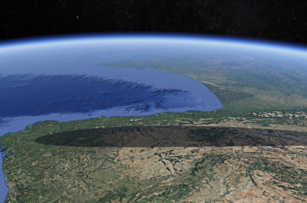
Alternatively, we can use Google Earth and take advantage of its cartographic projection in the form of a sphere to highlight the effect produced by the eclipse on a planetary scale and where curved and distorted geometric shapes take on more realism and meaning. An eclipse is still the result of the interference of light between two spheres projected on another sphere. In this context, "flat" projections lose the coherence of a spherical projection. The result can be seen as follows:
Figure 10: Map of the shadow areas created by the eclipse in Google Earth. Source: Done by datos.gob.es.
When integrating these visualizations into a web environment, Javascript libraries such as Leaflet or D3.js are of great help, since with a few lines of code you can create a map with the polygons contained in a GeoJSON, and customize the styles of that polygon in an easy and intuitive way. In the case of Leaflet, the next image shows the extent of the shadow area on a satellite projection. The corresponding code for the creation of this map can be found in an Observable notebook.
Figure 11: Map of the shadow zones created by the eclipse in Leaflet. Source: Done by datos.gob.es.
In the case of D3.js, we took advantage of the extensive library of cartographic projections to create a globe and, as in the case of Google Earth, give that planetary perspective that is, without a doubt, more realistic to understand the nature of an eclipse and the combined effect of the spherical geometries involved. In the following figure you can see the trace of the shadow area chosen for this exercise. To replicate this map you can use the code of the corresponding Observable notebook.
Figure 12: Map of the shadow areas created by the eclipse created with D3.js. Source: Done by datos.gob.es.
Lessons learned
In this data exercise we have learned how to read a . TIFF or . GPKG file, extract the relevant information, dump the data on structures such as xarray or GeoPandas, make a preliminary map without leaving Python, export the data in GeoJSON format and, finally, explore various tools depending on the environment we need for the visualization project. In this way, we have managed:
Gain familiarity with different geographic information formats such as . TIFF, . GPKG, or . SHP. This allows us to take advantage of the wealth of available formats, have the same geographic information represented in different forms, and thus enable the use of a plethora of tools to represent the data.
Read .TIF files through Python both for their graphic representation and for their transformation into valid formats to create visualizations on the web. In this process we also learn how to convert geographic data, going from input . TIFF and . GPKG files to output files in a manageable format suitable for web environments such as the GeoJSON format.
Delimit areas of interest from files with a wide spatial coverage, to focus on specific populations or regions and to be able to transmit a specific message when communicating relevant information. Specifically, we learn to cut out georeferenced information in TIFF format on a specific contour such as the boundaries of a municipality and to discard any data that is outside that contour.
Use the Cartopy and Matplotlib Python libraries to preview the information contained in a TIFF file.
Create a globe where the shadow area of an eclipse can be visualized using Google Earth or D3.js, providing a visualization with greater astronomical rigor.
Explore different visualization alternatives thanks to the diversity of tools available. Specifically, we take a tour of the entire spectrum of complexity of spatial visualizations, from intuitive tools such as GoogleEarth, with which the public is already familiar thanks to GoogleMaps, to code tools such as Python or Javascript through D3.js.
Conclusions
This data exercise has allowed us to move from formats commonly used in professional geographic information systems environments to more manageable ones to be able to create our own maps, either with the help of popular applications such as KeplerGL or GoogleEarth, or with Javascript libraries for integration into web projects.
We have also seen how with a few lines of code we can manipulate the input data to focus on regions of interest, select certain time intervals or customize maps to our liking and choice.
Next steps
The next steps proposed to deepen the analysis are:
Explore NetCDF or KML/KMZ formats, also georeferenced, to have greater control and mastery over the most popular data formats in geospatial mapping and analysis.
Compare the astronomical characteristics of the 2026 eclipse with those of 2027 and 2028, also available in the CNIG database accessible in the datos.gob.es Data Catalog .
Represent variables that have not been shown in this exercise, such as ephemeris or parameters such as the duration, elevation or azimuth of the celestial bodies involved in the eclipse.
Areas of application
The result of this data visualization exercise applies and appeals to the following areas of data analysis:
Journalistic: for the dissemination of accurate information regarding solar eclipses.
Scientific: once the data are accessible, all the astronomical variables included in the CNIG dataset can be explored and a much more complete portrait of the astronomical phenomenon can be made than the one described in this exercise
Analytical: the exercise has been limited to the most traditional visualization based on maps and cartographies. Exploring other forms of visualization with such an attractive dataset can encourage creativity and innovation when representing this type of event.
Science and technology
Introduction
In 2018, the company Uber created a tool to visualize geospatial information and to be able to graphically represent thousands of location points, as well as trajectories in a wide time range. This tool became public domain under the name KeplerGL and, today, it is available as open source for easy mapping.
KeplerGL allows you to represent georeferenced information in a web interface without the need to use tools such as ArcGIS or QGIS, or any other software that requires installation on the computer or complex updates.
KeplerGL offers a wide variety of representation shapes, from conventional dots or rectangles to hexagonal binning or heat map clustering forms, to more sophisticated mesh systems such as H3.
The entire range of graphic elements comes with a very complete series of customization options, both in size and color through to value ranges. The background cartography itself that is used to reference the information we want to visualize also has a whole catalog of options, including light and dark backgrounds or satellite images of the visible spectrum.
In this exercise we will visualise georeferenced information related to the seismic activity of the eruption of the La Palma volcano around September 2021. This information was reflected in various ways in several infographics in the state media, where the epicentres of the earthquakes were geolocated taking the island of La Palma as a reference. In Figure 1 we see the same type of map, in which circles are superimposed on a background cartography, and where the radius of the circles is proportional to the seismic activity. In this exercise we will learn how to make maps similar in content and style quickly and intuitively thanks to KeplerGL.
Figure 1: Map shown in various media with the epicentres of seismic activity prior to the eruption of the La Palma volcano. (a) Antena3, (b) Telemadrid, (c) La Vanguardia and (d) ElDiario.es
To create the seismic activity map, we have two options depending on the level of detail and processing we want to perform:
The first option is to use the data downloaded directly from the data portal as it is. The Dataset section provides a link to a .CSV file containing all the data needed to create the map and complete the exercise without programming or writing code.
The second option is to process and filter the data using Python if we want to familiarize ourselves with a few simple lines of code and select variables or time intervals of interest. Access to the GitHub repository and the Google Colab notebook for reading, selecting variables, and applying filtering criteria to obtain a subset of data can be obtained through the following links:
Access the Github repository
Access the GoogleColab notebook
Dataset
In this exercise we are going to use open data from the Cabildo Insular de La Palma collected during the seismic activity before and after the volcanic eruption on La Palma in 2021, and which are available here:
https://datos.gob.es/es/catalogo/l03380010-terremotos
In this dataset we find the record of each of the points where seismic activity was detected during those days, as well as, among others, the following metrics that characterize their geological properties:
Metrica
Descripción
ID
Identifier associated with each event
Datetime
Date and time of each event
ErrTime
Error associated with registration time
RMS
Root Mean Square Spread Time
Latitude
Latitude coordinate in degrees
Longitude
Longitude coordinate in degrees
Az
Azimuth degree
Depth
Event Depth in Kilometers
ErrDepth
Error associated with depth measurement
Nsta
Number of stations used to measure the event
Gap
Greater azimuth difference between adjacent stations
Author
Body responsible for measurement
Magnitud
Seismic magnitude of the event
IntensMax
Maximum intensity of the event
Localización
Location
TipoMagnit
Type of magnitude
XUTM
Longitude coordinate in the UTM system
YUTM
Latitude coordinate in the UTM system
GlobalID
Event ID
For the creation of the map we will focus on the variable associated with seismic activity: magnitude, as well as the longitude and latitude of each point and the date and time of each event.
Development Process
1. Access to the web interface
As we mentioned in the introduction, KeplerGL does not need to be installed on the computer, but can be accessed through the Internet to its interface. Therefore, the first thing we will do is open a browser and access the KeplerGL website through the domain:
https://kepler.gl/
Once on the home page we will click on Get Started to be able to upload the data and start creating our map.
As we can see in Figure 2, KeplerGL includes other options, such as accessing data that is stored in a database or directly querying the Github code, especially useful for developers or for integrating KeplerGL into other applications. However, in this case we will focus on the simplest option: uploading our data directly to the interface.
Figure 2: KeplerGL main screen where we are offered an example of visualization, as well as the option to start the process of creating our map.
2. Loading data on the page
On the data upload page we have the usual dialog box to be able to upload our data. As we can see in Figure 3, KeplerGL accepts different formats:
CSV: the traditional format with values, usually separated by commas.
JSON: alternative to CSV with structured entries in list and object format
GeoJSON: Geometric shapes structured like a JSON.
Arrow: Column-structured data for the Apache Arrow application.
Parquet: Column format for large amounts of data.
At this point, we will upload the data we obtained directly from the portal or the filtered data we created using the Python code in the Github repository and the Google Collab notebook. Both options are valid for creating the maps.
Figure 3: Dialog box for uploading files, either by selecting them from the computer or by dragging them directly into the browser.
3. Visualization
KeplerGL allows us to represent geographic information through various elements, such as points, grids, hexagon distributions, heat maps, as well as project all these shapes in three dimensions. Figure 4 details the different types of visualization possible that the tool offers.
Figure 4: Options for displaying georeferenced information, including points, trajectories, lines, boxes, hexagons, polygons, clusters, icons, heatmaps, H3 cells, three-dimensional, trips, S2 cells, vector, and rasters.
Below we see in detail the characteristics of the visualization forms that we can explore with this dataset.
3.1 Dots
Within the points we can parameterize the following variables: spot color, dot edge, additional magnitude associated with radius, radius dimensions, tags, tooltip with information, interaction between overlays or transparency.
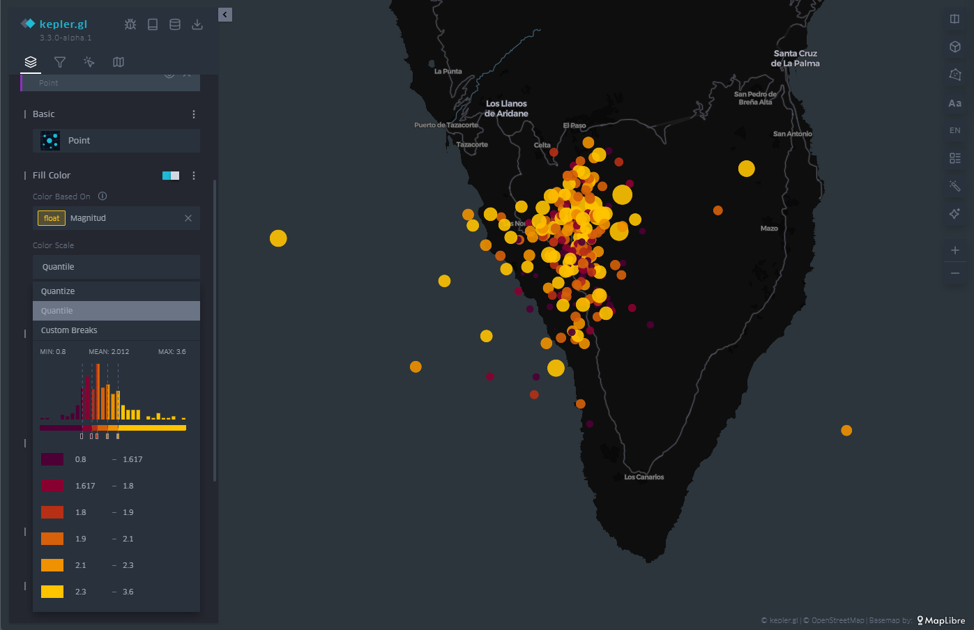
In Figure 5 we can see the direct application of the representation by points. KeplerGL identifies both latitude and longitude automatically to place each of the points on the plane. From there draw a circle with a certain radius and assign a color depending on the intensity of the magnitude.
In the control panel on the left, you can control both the radius of the circles and the color palette, and apply the options you like best to represent the intensity. Being able to play with both parameters would allow us to add another axis of information to the visualization. In this case, for simplicity's sake, we leave this representation as it is, exploring only the color and size.
Figure 5: Map with the earthquakes on the island of La Palma represented by points. The color is proportional to the magnitude of the earthquake and the radius remains constant.
3.2 Grid
In the same way that KeplerGL identifies latitude and longitude to place circles, it is also able to average magnitude values in cells. These cells can encompass one or more points, and KeplerGL assigns a color that represents their value based on the average value, as we see in Figure 6.
As with dots, the dialog box on the left allows you to change the color palette, increase or decrease the size of cells to average over larger or smaller areas. Likewise, the scale of values on which the assignment of each of the colors of the scale is based is also subject to customization, depending on the range of values that we want to highlight in the visualization.
Figure 6: Map with the earthquakes on the island of La Palma represented by a mesh. The color is proportional to the magnitude of the earthquake.
3.3 Hexbin
Similar to the cell mesh, hexbin is an acronym for hexagonal binning, i.e., averaging values over hexagon-shaped cells. Unlike rectangular cells, hexagon-shaped cell packing responds to more compact structures, similar to those that can be observed in the organization of particles or atoms in the formation of solid-state structures.
The hexbin has the same properties that we have seen in the case of the cell mesh, that is, we can change the size of the hexagonal cell so that it occupies a larger surface area on average, we can also change the color palette and also the range of values on which each color interval acts. An example of hexagonal binning is found in Figure 7.
Figure 7: Map with the earthquakes on the island of La Palma represented by hexagons. The color is proportional to the magnitude of the earthquake and the hexagon adds the points that cover its extension.
3.4 Heatmap
The last of the representations that we will see on the map is the heat map. The heatmap is nothing more than a contour diagram, where each contour corresponds to a certain range of values. At the moment when the number of contour lines is very high, we get that feeling of continuity that evokes the heat map.
In this case, both the chosen color palette with its number of levels and the radius over which the values are averaged are customizable through the options in the menu on the left. In Figure 8 we have an example, where the density of events emerges naturally with this type of representation.
Figure 8: Map with the earthquakes on the island of La Palma represented by a heat map. The color is proportional to the density of seismic events.
3.5 Three-dimensionality
Finally, in geographical representation we have the possibility of using the z-axis, or vertical axis, to add or redound information in that dimension. To do this, we have the option called "Height" in the menu on the left. The "Height" option applies to both circles and cell meshes, where it affects the polygon that defines each of the cells.
In this way, we project another magnitude of our choice onto the vertical, which complements the magnitude already represented by the color of the cells or circles on the plane, as illustrated in Figure 9.
Figure 9: Map with the earthquakes on the island of La Palma represented by rectangles. The height and color is proportional to the magnitude of the earthquake.
3.6 Time Filter
As you can see in Figure 10, in the upper left menu we find a very useful tool such as the time filter. When, as in this case, we have temporal information about the events, through the date field, we can use that information axis to filter the information we want to represent and focus on those days or times of greatest interest for our analysis and visualization project.
The filter tool allows you to choose the magnitude on which we are going to make the filtered selection. Once chosen, a histogram is displayed at the bottom in which we can see at a glance the distribution of the number of dots that correspond to each date. In Figure 10 we can see the histogram at the bottom.
This tool allows you to not only select a day but also a time slot. Sliding that time interval along the histogram allows us not only to see a certain period of interest, but also to make an animation that automatically moves that time interval throughout the entire time series.
This feature makes this filter a very attractive option to be able to create in seconds what is known as storytelling, that is, an easy and very intuitive animation.
Figure 10: Maps with the earthquakes on the island of La Palma through points with a temporal filter applied to the entire data sequence at the bottom. The half-height interval in the histogram specifies the temporal length.
As an example of animation we can see in Figure 11 a video showing the filter tool and how the window we define goes through the histogram. This animation focuses on the days before and after the volcano's eruption on September 19, 2021, as well as all the seismic activity that followed the volcano's eruption well into 2022.
Access the KeplerGL earquake activity motion map
Figure 11: Sequence of seismic activity detected before, during and after the volcanic eruption on the island of La Palma around September 2021.
3.7 Legend
As illustrated in Figure 12, in the menu on the right we have different options, such as arranging the cartographic projection in three dimensions or, in the lower right corner, activating the appearance of a legend.
The legend is associated with the variable that we have chosen to represent the points, in this case, the magnitude. The ranges are predefined according to the ranges that we defined when we created the ranges in the color scale of the points.
Figure 12: Legend of the color code and values used for the point representation, in line with our interval definitions in the point representation configuration.
3.8 Background Mapping
Depending on the event we represent on the map, it is convenient to use different types of background cartographies for a better understanding of the message that we are trying to convey through the visualization. Depending on the audience and context, the information provided by the background map can be more or less useful. If, as in this case, we only want to transmit geological information, its relevance is less. If, on the other hand, we also want to describe civil infrastructures that may be affected by earthquakes, it will be necessary to incorporate a basic cartography.
In this way, KeplerGL also offers a whole series of background cartographies, mainly divided into two families: those with a dark background and those with a light background. Here it is worth remembering that the human eye perceives small details better on a dark background, and interprets large shapes better on a light background. In the case of earthquakes and the scale at which we are representing them, it is advisable to use a dark background, as we will be able to discern distances and details more accurately.
To select the different background maps, go to the icon at the top of the left panel, and from the drop-down menu you can choose the one that suits you best. Figure 13 shows the different types of maps.
Figure 13: Different background cartographies in KeplerGL for the representation of seismic activity on the island of La Palma in September 2021: Positron (a), Satellite (b), Voyager (c) and Light (d).
4. Export the map
Finally, once we have made our map, we can export the result through the download icon located at the top of the menu on the left. Once that icon is selected, we can save the map as an image.
The options offered are: the size by the ratio of the image with respect to its horizontal and vertical dimensions, the resolution linked to that ratio that we have selected and the option to incorporate a legend in the output image, as shown in Figure 14.
Figure 14: Dialog box to export the map as an image. Note the selection of the box to show the legend, as well as the selection of a panoramic format with space to incorporate infographic elements into other content later.
Additionally, there is the possibility of sharing the map with all its interactivity through registration in Dropbox or Carto, if the intention is to disseminate the map through other channels beyond a static image.
Lessons learned
In this exercise we have learned how to create a map in a simple and intuitive way with the help of KeplerGL. Specifically, we have learned to:
Upload a file through the KeplerGL web interface.
Represent georeferenced information in different ways.
Learn how to use a temporal filter on the data series and create an animation for dissemination as a video.
Add a legend and handle the values that that legend reflects.
Customize each of the ways of visualization in detail.
Export the resulting map with a certain degree of customization.
Conclusions and next steps
The world of cartography has always needed prior knowledge about projections, reference systems, georeferenced data formats and above all the installation of specific software to create maps. Thanks to the development of web products, one of these projects allows us to create maps in a very simple way and can be a very powerful tool when it comes to creating maps without the need for much prior knowledge and with a high degree of customization.
From this point on, more sophisticated tools can be explored that require either general knowledge or programming knowledge to be able to make maps with Leaflet or with D3.js, depending on the audience and the application in which we want to frame the map.
Areas of Application
The creation of simple maps has many fields of application, since cartography in general turns out to be one of the clearest and most popular forms of visualization thanks to its use since the origin of civilization. Proposed areas include:
Journalism newsrooms: reacting to specific events such as natural disasters or large databases of georeferenced events can be easier thanks to tools such as KeplerGL.
Corporations: Location of volumes associated with specific points of geography can be read intuitively with the creation of maps that can summarize large amounts of data.
Applications: Integrating maps within applications often helps both the information and interactivity layers to explore the performance and outcome of a product at different scales.
Science and technology
Energy
Economy
Introduction
In recent years, we have seen how generative artificial intelligence has ceased to be a technical curiosity and has become an everyday tool in the workflow of data professionals. However, an important question remains: how does this technology translate into a real process of open data analysis?What changes in practice when an analyst works "alongside" a language model rather than alone?
This post documents a practical exercise carried out with data published on the datos.gob.es portal: the price analysis of the more than 11,000 service stations in Spain. Unlike other exercises published in this space, the analysis has not been carried out manually line by line, but has been carried out in an agentic environment: a conversational interface supported by a large language model (LLM) and a coding system assisted by artificial intelligence. In practice, this means that instead of writing the analysis code ourselves, we describe to the system in natural language what we want to obtain, and it implements it.
The objective of this post is twofold. On the one hand, to explain the analysis itself: what questions we ask ourselves about the data, what technical problems we find and what conclusions we draw. On the other hand, to reflect on the method: how an analysis process is structured when working with an AI co-pilot, what interaction patterns work best, and where the limits of automated assistance are.
Methodological note: to carry out this exercise we have used a Spec Driven Development (SDD) methodology, which guides the AI through a structured process with the aim of preventing the conversation from losing the focus of the exercise. The detailed explanation of this methodology is beyond the scope of this post, but the reader will find in the repository specifications, technical plans and checklists that document it.
Accesses the GoogleColab notebook
Accesses the GoogleColab notebook
In this video, the author explains what you will find on both Github and Google Colab.
The process: a classic, AI-assisted flow
Before entering into each phase, it is useful to describe the general outline of the work. The analysis follows five common stages in data science—ingestion, cleansing, exploration, variable engineering, and impact analysis—but introducing a conversational pattern with AI in each of them.
That pattern can be summarized in five steps:
Describe the problem in natural language.
Propose a first solution (AI does it).
Question the assumptions of that proposal (the human analyst does it).
Refine the solution until it is robust.
Document the pattern for reuse in future projects.
Below, we will see, phase by phase, how this pattern materializes in the analysis of fuel prices. Each section begins by explaining the conceptual challenge, continues to describe how we approach the resolution with the assistance of AI, and ends by showing the resulting code and lessons learned.
Phase 1: Robust data ingestion from a public API
The challenge: public APIs that don't always respond as expected
Notice to reader: This phase goes into some technical detail about API integration, SSL errors, and backup strategies. If your profile is more analytical than developmental, you can skim through the code block and focus on the Approach and Reflection sections, where the underlying idea—how to design fault-tolerant ingestion—is explained without going into implementation details.
Downloading data from the API of the Ministry for Ecological Transition is conceptually simple: an HTTP GET request to a known endpoint should return a JSON file with approximately 11,000 service stations. In practice, however, public APIs present common difficulties that any analyst ends up encountering sooner or later:
Expired or misconfigured SSL certificates, which cause SSLError errors.
Blocking of IPs from cloud servers (Google Colab, AWS, etc.), interpreted as suspicious traffic.
Unstable servers, with variable response times and sporadic timeouts.
Inconsistencies in documentation, for example, when a JSON response is described but the server returns XML.
The key question is: how do we design an intake system that tolerates these problems rather than failing at the first hurdle?
The Approach: A Tiered Backup Architecture
In software engineering, critical systems don't depend on a single component. When one channel fails, there is a fallback channel. Applying this logic to data ingestion is especially useful when working with public sources over which we have no control.
For this exercise, we designed a three-pronged strategy:
First attempt — requests with permissive configuration: we make the HTTP request with the standard Python library, but configuring a User-Agent that simulates a real browser and disabling SSL verification. This solves a good part of the certificate problems.
Second attempt — curl from shell: If requests fails, we invoke curl as a thread. The reason is that curl uses a different TLS stack than Python and does not send the same certificates, which allows certain types of blocking to be circumvented.
Third attempt — demo data: if all else fails, we generate a synthetic set of 11,000 service stations with realistic distributions. This ensures that the notebook is always executable in an educational context, even if the API is down.
The basic reasoning is simple: each method circumvents a different type of network failure, and their combination provides robustness. Below, we show the code that implements this architecture.
The resulting code
The following excerpt illustrates how the three levels of support materialize into a single function. The try/except clauses allow the failure of each method to be detected and automatically moved to the next one:
def descargar_datos_api(url):
"""
Download data with triple backup:
1. requests with verify=False (circumvents SSL issues)
2. curl -k (alternate TLS stack)
3. Synthetic data (performance guarantee)
"""
# Attempt 1: Requests with browser headers
Try:
sesion = requests. Session()
sesion.headers.update({
"User-Agent": "Mozilla/5.0 (Windows NT 10.0; Win64; x64)"
})
response = sesion.get(url, timeout=45, verify=False)
return response.json()
except Exception as e_requests:
print(f"[Respaldo 1] requests ha fallado: {e_requests}")
# Attempt 2: curl as thread
Try:
resultado = subprocess.run(
["curl", "-s", "-k", url],
capture_output=True, timeout=45, text=True
)
return json.loads(resultado.stdout)
except Exception as e_curl:
print(f"[Backup 2] curl has failed: {e_curl}")
# Attempt 3: Demo Synthetic Data
print("[Backup 3] Using demo data")
return generar_datos_demo_gasolineras(11000)
Reflection: where AI adds value in this phase
Iteration with AI didn't produce the previous code in one attempt. The actual process was more interesting: we posed the problem ("the API sometimes rejects requests, I need backups"), the AI proposed an initial solution, and the breakthrough came from questioning that proposal. The question "why should curl work if requests has already failed?" forced the model to explain the differences between the two TLS stacks, which in turn allowed us to validate that the solution had real technical merit, it wasn't just "try the same thing twice".
A reasonable estimate: Solving this problem through pure trial and error would have taken about two to three hours of debugging. With assisted iteration, we tackle it in about thirty minutes.
Phase 2: Cleaning with domain knowledge
The challenge: real data is never perfect
Once the data is downloaded, the least visible but most decisive work of any analysis begins: cleaning and preparation. The quality of the final result depends to a large extent on the care put into this stage. In the case of fuels, the most common inconsistencies are:
Non-standard textual variants: The trademark "MOEVE" may appear as "MOEVE", "Moeve" or "moeve" in different registers. To a person they are obviously the same brand, but in an aggregation by groupby they appear as three separate categories.
Incorrect geographical coordinates: points located outside Spanish territory (remote islands, fragments of Morocco, capture errors).
Inconsistent decimal separators: Prices coded as "1.349" with a comma, which require explicit conversion before you can trade them.
Conversions that introduce null values: pd.to_numeric(..., errors='coerce') is very useful, but it generates silent NaN that can break subsequent analyses.
The central question of this phase is: how do we translate human domain knowledge into code rules?
The approach: validation organized in layers
Instead of cleaning up "as it happens," it's a good idea to organize validation rules into layers, each with a clear responsibility:
Layer
Liability
Example
Types
Conversion and coercion at appropriate rates
Price as float, date as datetime
Ranks
Values within reasonable limits
Price between €0.5 and €3.0 per litre
Semantics
Domain consistency
Coordinates within Spain, standardised marks
Figure 1. Validation table organised by layers. Source: own elaboration - datos.gob.es
The question that each layer must answer is always the same: does this value make sense in the context of Spanish service stations? The novelty compared to a manual flow is that here we describe the rules to the AI in natural language and let it translate them into panda code. We retain the responsibility of defining what is valid and what is not.
The resulting code
The next block implements the three validation layers sequentially. It should be noted that the list of brand aliases (CEPSA → MOEVE) reflects specific business knowledge – the rebranding of CEPSA to MOEVE in 2023 – that AI could not infer on its own; it is information provided by the analyst. This is a very clear example of the contribution of human knowledge that is difficult to achieve by AI:
def validar_y_limpiar_carburantes(df):
# Layer 1: Type Normalization
df['price'] = (
df['precio'].astype(str)
.str.replace(',', '.')
.astype(float)
)
df['March'] = df['March'].str.upper().str.strip()
# Layer 2: Rank Validation
df = df[(df['price'] >= 0.5) & (df['price'] <= 3.0)]
df = df[
(df['latitude'] >= 27.5) & (df['latitude'] <= 43.8) &
(df['longitude'] >= -18.2) & (df['longitude'] <= 4.4)
]
# Layer 3: Semantic coherence (business knowledge)
aliases = {'CEPSA': 'MOEVE'} # Rebranding 2023
df['tag'] = df['tag'].map(lambda x: aliases.get(x, x))
# Null audit
null = df[['price', 'latitude', 'longitude', 'mark']].isnull().sum()
if nulos.sum() > 0:
print(f"Attention: null values have been detected:\n{null}")
return df.dropna(subset=['price', 'latitude', 'longitude'])Reflection: the division of work between AI and the analyst
This phase is especially revealing of the type of collaboration that AI enables. The more technical rules (type conversion, null detection, capitalization normalization) are practically automatic: just describe the problem and the model proposes a correct implementation. On the other hand, the rules that depend on the domain (that the Canary Islands have a logistics cost overrun of 5%, that CEPSA and MOEVE are the same brand after the merger, that a price of less than €0.5 is probably a loading error) must be specified by the human analyst.
The lesson learned is important: the quality of cleanliness depends directly on the domain knowledge that the analyst provides. AI speeds up deployment, but it doesn't invent context. That's why the reusable pattern is the same in any project: describe your domain in detail, let the AI write the validations, and verify yourself that the results are consistent.
Phase 3: Visual Exploratory Analysis (EDA)
The challenge: turning numbers into intuitions
With 11,000 clean records already in memory, the next step is to answer the business questions that prompted the analysis. In this case, we ask four specific questions:
Which provinces have the most expensive fuels?
Is there a relationship between geographical location (latitude and longitude) and price?
Are there significant differences between brands?
How are prices distributed (mean, median, outliers)?
The technical challenge is not complex – pandas and matplotlib solve any of these questions – but the methodological challenge is: choosing the right visualization for each question. A poorly chosen chart can hide as much as an incorrect aggregation.
The approach: each question determines its graph
In exploratory analysis there is a natural correspondence between the type of question and the most appropriate visualization. It is worth keeping this in mind before writing a single line of code:
Question
Proper Visualization
Reason
Ranking?
Neat bar chart
Allows you to compare ordered values
Spatial relationship?
Scatter with color scale
Shows correlation in two dimensions
Distribution and atypical?
Box plot
Reveals median, quartiles and outliers
Differences between groups?
Box plot o violin plot
Compare distributions simultaneously
Figure 2. Table showing the natural correspondence between question type and the most appropriate visualisation. Source: own elaboration - datos.gob.es
The goal is not to produce flashy graphics, but graphics that answer specific questions. This is a seemingly obvious idea, but it's worth remembering: in practice, it's common for viewings to be generated by inertia, without being clear about what you want to show.
The resulting code
Below, we show one of the graphs as an example, the price ranking by province. The structure is always the same: statement of the graphic, aesthetic configuration, and a brief comment interpreting the result:
# Question 1: Which provinces are the most expensive?
top_provincias = (
df.groupby('province')['price']
.mean()
.sort_values(ascending=False)
.head(12)
)
fig, ax = plt.subplots(figsize=(12, 6))
top_provincias.plot(kind='bar', ax=ax, color='steelblue')
ax.set_title('Average fuel price by province (Top 12)',
fontsize=14, fontweight='bold')
ax.set_ylabel('Price (€/litre)')
ax.set_xlabel('Province')
plt.xticks(rotation=45, ha='right')
plt.tight_layout()
plt.show()
# Finding: the three most expensive provinces are island or coastal
# (Balearic Islands, Canary Islands, Tarragona). Hypothesis: the logistics cost
# and the distance from distribution hubs raise the price.In the case of the geographic scatter, we apply additional segmentation – mainland, Balearic and Canary Islands – to simultaneously visualize location and insularity. This segmentation revealed a pattern that no numerical aggregation had clearly shown: island stations have systematically higher prices, a finding probably attributable to shipping costs. Insight did not emerge from a calculation, but from visualization.
Reflection: The AI blind spot
This phase highlights an important limitation of the model: the AI does not see the graphical result. You can suggest the right type of visualization, write the code correctly, and propose a color palette, but you can't judge whether the axis scale is appropriate, whether the dot density saturates the graphic, or whether the labels overlap. All these validations remain the responsibility of humans.
In practice, this means that the EDA phase is the one that requires the most iteration between person and machine: the AI writes, the analyst observes, identifies a visual problem ("this axis does not show the variation well"), and describes the correction ("sets the Y-axis to [precio_min0.95, precio_max1.05]"). The reusable pattern is clear: a clear question, a suitable chart type, and human visual validation.
Phase 4: Feature engineering
The challenge: capturing variation with new variables
Exploratory analysis identifies patterns, but rarely explains them. To understand what factors influence the price , it is necessary to construct new variables (features) that capture specific hypotheses about market dynamics. In this exercise we formulate three hypotheses:
Temporary: Does the day of the week influence the price? Is it more expensive to refuel at the weekend?
Geographical: Does the distance to an economic hub (in this case, Madrid) have an influence?
Regional: Are there structural differences between the north, centre and south of Spain?
Variable engineering consists precisely of translating these hypotheses into calculated columns that the rest of the analysis can use.
The approach: every variable, a testable story
A good variable should tell a clear story. It is not enough to calculate a number: you have to be able to explain what question you are trying to answer. In our case:
es_fin_semana (0/1): Does the price change on Saturday and Sunday?
distancia_a_madrid (km): Does fuel become more expensive when moving away from the logistics hub?
Region (North/Central/South): Are there structural gaps between regions?
Each of these three variables is, in reality, an empirical question disguised as a column. If the variable does not explain anything when we cross it with the price, we simply discard it.
The resulting code
We implemented all three variables into a single function. The most technically interesting is the distance to Madrid, which requires Haversine's formula to calculate distances on the Earth's surface taking into account the curvature of the planet:
from math import radians, cos, sin, asin, sqrt
def crear_features_carburantes(df):
# Temporal variable
df['es_fin_semana'] = (
df['fecha'].dt.dayofweek.isin([5, 6]).astype(int)
)
# Geographic variable: distance haversine to Madrid
madrid_lat, madrid_lon = 40.4168, -3.7038
def haversine(lat, lon):
lat, lon = radians(lat), radians(lon)
m_lat, m_lon = radians(madrid_lat), radians(madrid_lon)
chisel = years - m_lat
dlon = lon - m_lon
a = sin(dlat/2)**2 + cos(m_lat) * cos(lat) * sin(dlon/2)**2
return 6371 * 2 * asin(sqrt(a)) # radius of the Earth in km
df['distancia_a_madrid'] = df.apply(
Lambda R: haversine(r['latitude'], r['longitude']), axis=1
)
# Variable regional
def region(lat):
if lat >= 42: return 'Norte'
if lat >= 39: return 'Centro'
return 'On'
df['region'] = df['latitud'].apply(region)
return dfReflection: proposing variables with argument, not just code
At this stage, AI provides particularly high value, but not in what you might think at first glance. What is really useful is not that he writes Haversine's formula – any technical reference contains it – but that he proposes candidate variables with argumentation behind them. When we asked "what features could capture the price variation?", the proposal was accompanied by reasoning: Madrid was suggested as a hub because it is the most efficient and stable market, and therefore deviations from its price work as an approximation to logistical friction.
That reasoning is what is valuable: not the formula, but the justification. Pure trial-and-error would have taken three or four hours exploring variables to find the useful ones; With assisted iteration, we arrive at a reasoned set in about forty-five minutes.
Phase 5: Analysis of the impact of the variables
The challenge: quantifying the real contribution
Building variables is one thing; Showing that they really explain something is another. In this last phase of the analysis, we evaluated the effective impact of each of the three variables created, combining two approaches: a numerical measure (correlation or difference in means) and a visual representation that allows us to interpret the result at a glance.
The approach: two complementary approaches
For each variable, we calculate:
A numerical measure that quantifies the effect (Pearson correlation for continuous variables; mean difference for categorical variables).
A visual representation that allows the magnitude of the effect to be interpreted and non-linear relationships to be detected.
The crossing of both approaches is what gives reliability to the result. A high correlation without a visualization to support it can be misleading (e.g., if it is dominated by outliers); A suggestive visualization without metrics can lead to overinterpretation.
The resulting code
As an example, we show the impact analysis of the distance to Madrid. First we calculate the correlation, then we segment it into quartiles to make the relationship visually interpretable:
# Numerical Measurement
correlation = df['distancia_a_madrid'].corr(df['price'])
print(f"Correlation (distance to Madrid → price): {correlation:.3f}")
# Visual representation by distance quartiles
df['cuartil_distancia'] = pd.qcut(
df['distancia_a_madrid'], q=4,
labels=['Q1 (near)', 'Q2', 'Q3', 'Q4 (far)']
)
precio_por_cuartil = df.groupby('cuartil_distancia')['precio'].mean()
fig, ax = plt.subplots(figsize=(10, 5))
precio_por_cuartil.plot(kind='bar', ax=ax, color='#2ecc71')
ax.set_title ('Geographical impact: average price per quartile distance to Madrid')
ax.set_ylabel('Average price (€/litre)')
plt.xticks(rotation=0)
plt.tight_layout()
plt.show()The emerging pattern of the complete analysis – comparing the three variables – is that the distance to Madrid is the most explanatory, followed by the region, and finally by the weekend effect, which in our study period turns out to be marginal. Together, the three variables explain approximately 60-70% of the price variation; The rest depends on factors such as the specific brand, the type of season (highway, urban, rural) and specific market events.
Reflection: not all variables have the same impact
One of the virtues of this structured analysis is that it reveals which of our initial hypotheses hold and which do not. In this case, the temporal (weekend) hypothesis turned out to be much weaker than expected, while the geographical hypothesis was clearly confirmed. Without this quantification step, we would have been able to continue assuming that all variables provide valuable information.
Synthesis: the technical lessons we take away
Throughout the five previous phases we have been accumulating solutions to specific problems. The following table summarizes the most reusable; Each is documented in greater detail in the repository's Prompts directory:
Phase
Problem
Solution
Reusable in
Intake
SSL or IP blocks in APIs
Triple respaldo: requests → curl → demo
Any public API
Intake
Inconsistent documentation
Structure validation + error handling
Government APIs
Cleaning
Textual variants in trademarks
.str.upper().str.strip() before grouping
Any categorical aggregation
Cleaning
Coordinates outside Spain
Bounding box [27.5–43.8, −18.2–4.4]
Geographical analyses in Spain
Cleaning
Compressed ranges in graphs
ax.set_xlim(min*0.95, max*1.05)
Viewing with narrow ranges
EDA
Choosing a chart type
Explicit Mapping Question → Graph
Any EDA
Features
Unjustified variables
Each feature responds to a testable hypothesis
Feature engineering in general
Analysis
Unquantified impact
Metric + side-by-side display
Any impact analysis
Figure 3. Summary table of solutions to specific problems. Source: own elaboration - datos.gob.es
Final Thought: What Makes AI a Good Co-Pilot
At the end of the exercise, we can draw some general conclusions about the use of generative AI to support data analysis. We divide them into two levels: where it adds value, and where it should not replace human judgment.
Where AI clearly adds value:
Rapid iteration. The cycle "describe problem – get solution – validate" is reduced from hours to minutes. This qualitatively changes the work dynamic: it allows us to test ideas that we would otherwise discard because of cost.
Lateral thinking. AI proposes alternatives that an analyst might overlook, such as the idea of using curl when requests fail. It does not always get it right, but it does expand the space of solutions considered.
Articulated documentation. AI is especially good at explaining the why of a technical decision, not just the what. This makes it easier for the resulting code to be readable by non-technical people.
Where human judgment is still essential:
Domain knowledge. The AI does not know that CEPSA and MOEVE are the same brand, nor that the Canary Islands have a structural logistical cost overrun. That information must be provided by the analyst.
Statistical validation. AI can suggest models, but the statistical validity of the analysis is a human responsibility.
Reading graphs. The AI doesn't see its own visualizations. The judgment on whether a graphic is legible, communicates what is intended and respects good visual practices is still human.
Business decisions. What to ask of the data, what to consider relevant, how to communicate the results to the organization: these are decisions that AI can support, but not replace.
In short, the idea that best sums up our experience is this: generative AI works better when it thinks with us than when it thinks for us. The exercise we present here was not to "ask Claude to do the analysis", but to have a structured conversation in which the AI proposed, the analyst questioned, the AI refined, and the analyst validated. The result of that conversation is a more robust, better documented, and more reusable analysis than we would have produced alone.
How to take advantage of this repository
The full code, prompts, and documentation are available in the project's public repository. Different profiles can take advantage of it in different ways:
If you study data analysis: open the notebook directly in Google Colab and go through each cell in order. For each visualization, please refer to the corresponding prompt in prompts/visualization/.
If you work as a data scientist: Check out specs/001-fuels-ia/plan.md, where architectural decisions and lessons learned are documented. Prompts/ snippets are reusable as is in other projects.
If you're interested in prompt engineering methodology: the "describe – question – refine – validate" pattern is documented on a case-by-case basis throughout the prompts. It is replicable in any domain: finance, health, marketing, or any open data analytics.
Conclusion
The exercise we have presented shows that generative AI, used judiciously, can significantly accelerate the analysis of open data without sacrificing methodological rigor. The five phases covered – ingestion, cleaning, exploration, variable engineering and impact analysis – remain the same as in a traditional flow, but the work dynamic changes: we go from writing code to describing intentions and validating results.
The total time spent was approximately forty hours, compared to the one hundred and twenty that would have required equivalent development without AI assistance. But more important than the time savings is the quality of the resulting product: a documented, reproducible analysis accompanied by a library of reusable prompts.
Generative AI doesn't relieve us of analytical responsibility, but it does allow us to spend more time on what really matters: asking the right questions, judiciously validating results, and communicating conclusions clearly. In short, to do better data science.
Content created by Alejandro Alija, an expert in digital transformation and innovation. The content and views expressed in this publication are the sole responsibility of the author.

Science and technology
Introduction
Every year there are tens of thousands of accidents in Spain, in which thousands of people are injured of varying degrees, and which occur in very different circumstances, both in terms of the type of road and the type of accident.
Many of the statistics related to these parameters are collected in the databases of the Directorate General of Traffic (DGT) and some of them in the catalogue hosted in datos.gob.es.
In this exercise, you will examine the content of the DGT accident database for the year 2024 in order to make a series of basic visualizations that allow us to quickly and intuitively see which are the facts to highlight regarding the incidence of accidents and their consequences in that year.
To do this, we are going to develop Python code that allows us to read and calculate basic metrics regarding the total number of victims, the particularities of the infrastructures as well as the different cases of accidents. And once we have this data available, we will visualize it using the Javascript D3.js library, which allows us both to represent data in its most traditional form and in more contemporary designs, common in the press, thus favoring a narrative that is fluid in style and coherent in content.
In the Python environment we will use commonly and frequently used libraries such as Numpy, for basic calculation - sums, maximums and minimums, and Pandas, to structure the data intuitively, facilitating both its organization and its transformation. We will also work with Datetime, both for the formatting of the input data in standard date types within the world of Python programming, and to add the data in an easy and intuitive way. In this way we will learn how to open any type of data file in . CSV, to structure it in an orderly way and to carry out basic transformations and operations in a simple way.
In the Javascript environment we will develop notebooks in D3.js thanks to the use of Observable, an open and free initiative, to be able to execute Javascript code directly in a web interface, and without having to resort to local servers or complex installations. In different notebooks we will create classic visualizations -such as time series on
Cartesian axes or maps- along with other proposals such as bubble distributions or elements stacked by categories.
In Figure 1 you can see the main stages of this exercise, from the reading of the data within the DGT file, to the operations and output variables in JSON format, which will in turn serve us in a Javascript environment to be able to develop the visualizations in D3.js.
Figure 1. Steps to be followed when performing this exercise, from reading the input CSV file, postprocessing the data with Python, creating an output in JSON format and ultimately displaying the information in D3.js
Access to the Github repositories, GoogleColab notebook and Observable notebooks is done via:
Access to the Github repository
Access to GoogleColab notebook
Access to Observable notebooks
Development Process
1. Reading the data file
The first step will be to read the DGT file containing all the accident records for the year 2024. This step will allow us to identify the fields of interest and especially in what format they are. We will be able to identify if any transformation is required, especially in the information of the date, as it is structured in the original file.
We will also see how to translate the codes of many of the categories offered by the DGT, so that we can make a real interpretation beyond the numbers of categories such as type of accident, type of road or ownership of the road.
Once we understand the structure and content of the data, we can start operating with it.
2. Calculating Metrics
The Pandas Python library allows us to operate with the different columns of data and perform basic calculations that will be representative enough to minimally understand the casuistry of accidents on Spanish roads.
In this section, three types of calculations will be made.
The first of these will be the calculation of the total number of victims per hour of the day for each of the days of the week. The DGT database is structured by day of the week, so we will also use this time scale to represent the data in a series. It should be noted that avictim is considered to be any person who has died or who is diagnosed as seriously or lightly injured.
The second calculation will be the sum of the total of accidents for different categories, such as road ownership, type of accident or type of road. This will allow us to see which are the conditions in which accidents are most frequent.
The third calculation will be the number of accidents per municipality. In this case we will carry out the calculation restricted to the province of Valencia as an example, and which would be applicable to any province or municipality of our interest. In this case we will observe the differences between urban and non-urban centers, as well as those municipalities through which the main communication routes pass.
3. Visualization Design
Once we have calculated the metrics of interest, we will develop four visualization exercises in D3.js. To do this, we will export the result of the metrics in JSON format and create notebooks in Observable. Specifically, we made the following visualizations:
Time series with the total number of casualties in each hour and day of the week, with an interactive drop-down menu to select the day of the week of interest. In addition to the curve that describes the number of victims, we will draw the uncertainty of all the days of the week on the background of the graph, so that the daily time series is framed in the context of the whole week as a reference.
Map of the province of Valencia with the total number of accidents by municipality.
Bubble diagram, with the different magnitudes of the different types of accidents with the total number of accidents in each case written in detail.
Stacked dot diagram, where we accumulate circles or any other geometric shape for the different road ownership and its total number of accidents within the framework of each ownership.
Mountain ridge diagram, where the height of each mountain represents the total number of victims on a logarithmic scale.
Viewing metrics
The result of this exercise can be seen graphically and explicitly in the form of visualizations made for the web format and accessible from a web interface, both for its development and for its subsequent publication. These visualizations are gathered as Observable notebooks here:
Access to Observable notebooks
In Figure 2 we have the result of the time series of the total number of victims with respect to the time of day for different days of the week. The time series is framed within the uncertainty of the total number of days of the week, to give an idea of the margin of variability that we can have depending on the time of day.
Figure 2. Time series of total accident casualties by time of day for all days of the week in 2024. The light blue background indicates the uncertainty associated with all the days of the week as context, with a drop-down menu to select the day of the week.
In Figure 3 we can see the map of the province of Valencia with a colour intensity proportional to the number of accidents in each municipality. Those municipalities in which no accidents have been recorded appear in white. Intuitively you can guess the layout of the main roads that cross the province, both the road to the east of the city of Valencia in the direction of Madrid and the inland road to the south of the city in the direction of Alicante
Figure 3. Map of the number of accidents by municipality in the province of Valencia in 2024.
In Figure 4 we see a geometric shape, the circle, associated with the types of accidents, with the detail of the number of accidents associated with each category. In this type of visualization, the most frequent accidents around the center of the diagram naturally emerge, while those that are minority or residual occupy the perimeter of the diagram to also give a round shape to the set of shapes
Figure 4. Bubble diagram of the number of accidents by accident type in 2024.
Figure 5 shows the traditional bar diagram, but this time broken down into smaller units, to refine the number of accidents associated with the ownership of the road where they have occurred. This type of diagram allows us to discern small differences between similar quantities, preserving the general message that we obtain from a calculation of these characteristics.
Figure 5. Bar diagram with dot discretization for the number of accidents by road ownership in 2024
Figure 6 shows the total number of victims on a logarithmic scale based on the height of each mountain for each type of road.
Figure 6. Mountain ridge diagram, displaying the total number of victims by each type of road in 2024.
Lessons learned
Through these steps we will learn a whole series of transversal skills that allow us to work with those datasets that are presented to us in CSV format in columns, a very popular format for which we can perform both their analysis and their visualization. These lessons are specifically:
Universality of reading and structuring data: the use of tools such as Python, with its Numpy and Pandas libraries, allows access to data in detail and structured in an orderly and intuitive way with a few lines of code.
Simple calculations in Pandas: the Python library itself allows simple but essential calculations for the preliminary interpretation of results.
Datetime format: through this Python library we can become familiar with the standard date format, and thus perform all kinds of transformations, filters and selections that interest us the most in any time interval.
JSON format: once we decide to give space to our visualizations on the web, learning the structure and use of the JSON format is very useful given its wide use in all types of applications and web architectures.
Spectrum of D3.js possibilities: this Javascript library allows us to explore from the most traditional and conservative to the most creative thanks to its principles based on the most basic shapes, without templates, templates or predefined diagrams.
Conclusions and next steps
We have learned to read and structure data according to the standards of the most widely used formats in the world of analysis and visualization. This exercise also serves as an introductory module to the world of D3.js, a very versatile, current and popular tool within the world of storytelling and data visualization at all levels.
In order to move forward in this exercise, it is recommended:
For analysts and developers, it is possible to dispense with the Pandas library and structure the data with more elementary Python objects such as arrays and matrices, looking for which functions and which operators allow the same tasks that Pandas does to be performed but in a more fundamental way, especially if we think of production environments for which we need the fewest possible libraries to lighten the application.
For the creators of visualizations, information on municipalities can also be projected onto existing cartographic databases such as OpenStreetMap and thus link the incidence of accidents to orographic features or infrastructures already reflected in these cartographic databases. For the magnitudes of the accident numbers, you can explore Treemap diagrams or Voronoi diagrams and see if they convey the same message as the ones presented in this exercise.
Areas of application
Los pasos descritos en este ejercicio pueden pasar a formar parte de cualquier caja de herramientas de uso habitual para los siguientes perfiles:
Data analysts: here are the basic steps for the description of a data file in CSV format and the basic calculations to be carried out both in the date field and operations between variables of different columns. These tools can be used to introduce you to the world of data analysis and help in those first steps when facing a dataset.
Scientists and research staff: the universality of the tools described here apply to a wide variety of data sources, such as that experienced in experimental sciences and observations or measurements of all kinds. These tools allow for a quick and rigorous analysis regardless of the field of knowledge in which you work.
Web developers: the export of data in JSON format as well as the Javascript code offered in Observable notebooks are easily integrated into all types of environments (Svelte, React, Angular, Vue) and allow the creation of visualizations on a website in a simple and intuitive way.
Journalists: covering the entire life process of a data file, from its reading to its visualization, gives the journalist or researcher independence when it comes to evaluating and interpreting the data by himself without depending on external technical resources. The creation of the map by municipalities opens the door to using any other similar data, such as electoral processes, with the same output format to show geographical variability with respect to any type of magnitude.
Graphic Designers: Handling visualization tools with a wide degree of freedom allows designers to cultivate all their creativity within the rigor and accuracy that data requires.
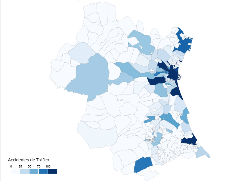
Science and technology
IA agents (such as Google ADK, Langchain and so) are so-called "brains". But these brains without "hands" cannot operate on the real world performing API requests or database queries. These "hands" are the tools.
The challenge is the following: how do you connect brain with hands in an standard, decoupled and scalable fashion? The answers is the Model Context Protocol (MCP).
As a practical exercise, we built a conversational agent system that explores the Open Data national repository hosted at datos.gob.es through natural language questions, smoothing in this way the access to open data.
In this practical exercise, the main objective is to illustrate, step by step, how to build an independent tools server that interacts with the MCP protocol.
To make this exercise tangible and not just theoretical, we will use FastMCP to build the server. To prove that our server works, we will create a simple agent with Google ADK that uses it. The use case (querying the datos.gob.es API) illustrates this connection between tools and agents. The real learning lies in the architecture, which you could reuse for any API or database.
Below are the technologies we will use and a diagram showing how the different components are related to each other.
FastMCP (mcp.server.fastmcp): a lightweight implementation of the MCP protocol that allows you to create tool servers with very little code using Python decorators. It is the “main character” of the exercise.
Google ADK (Agent Development Kit): a framework to define the AI agent, its prompt, and connect it to the tools. It is the “client” that tests our server.
FastAPI: used to serve the agent as a REST API with an interactive web interface.
httpx: used to make asynchronous calls to the external datos.gob.es API.
Docker and Docker Compose: used to package and orchestrate the two microservices, allowing them to run and communicate in isolation.
Figure 1. Decoupled architecture with MCP comunication.
Figure 1 illustrates a decoupled architecture divided into four main components that communicate via the MCP protocol. When the user makes a natural language query, the ADK Agent (based on Google Gemini) processes the intent and communicates with the MCP server through the MCP Protocol, which acts as a standardized intermediary. The MCP server exposes four specialized tools (search datasets, list topics, search by topic, and get details) that encapsulate all the business logic for interacting with the external datos.gob.es API. Once the tools execute the required queries and receive the data from the national catalog, the result is propagated back to the agent, which finally generates a user-friendly response, thus completing the communication cycle between the “brain” (agent) and the “hands” (tools).
Access the data lab repository on GitHub
Run the data pre-processing code on Google Colab
The architecture: MCP server and consumer agent
The key to this exercise is understanding the client–server relationship:
The Server (Backend): it is the protagonist of this exercise. Its only job is to define the business logic (the “tools”) and expose them to the outside world using the standard MCP “contract.” It is responsible for encapsulating all the logic for communicating with the datos.gob.es API.
The Agent (Frontend): it is the “client” or “consumer” of our server. Its role in this exercise is to prove that our MCP server works. We use it to connect, discover the tools that the server offers, and call them.
The MCP Protocol: it is the “language” or “contract” that allows the agent and the server to understand each other without needing to know the internal details of the other.
Development process
The core of the exercise is divided into three parts: creating the server, creating a client to test it, and running them.
1. The tool server (the backend with MCP)
This is where the business logic lives and the main focus of this tutorial. In the main file (server.py), we define simple Python functions and use the FastMCP @mcp.tool decorator to expose them as consumable “tools.”
The description we add to the decorator is crucial, since it is the documentation that any MCP client (including our ADK agent) will read to know when and how to use each tool.
The tools we will define in this exercise are:
buscar_datasets(titulo: str): to search for datasets by keywords in the title.
listar_tematicas(): to discover which data categories exist.
buscar_por_tematica(tematica_id: str): to find datasets for a specific topic.
obtener_detalle_dataset(dataset_id: str): to retrieve the complete information for a dataset.
2. The consumer agent (the frontend with Google ADK)
Once our MCP server is built, we need a way to test it. This is where Google ADK comes in. We use it to create a simple “consumer agent.”
The magic of the connection happens in the tools argument. Instead of defining the tools locally, we simply pass it the URL of our MCP server. When the agent starts, it will query that URL, read the MCP “contract,” and automatically know which tools are available and how to use them.
# Ejemplo de configuración en agent.py
root_agent = LlmAgent(
...
instruction="Eres un asistente especializado en datos.gob.es...",
tools=[
MCPToolset(
connection_params=StreamableHTTPConnectionParams(
url="http://mcp-server:8000/mcp",
),
)
]
)3. Orchestration with Docker Compose
Finally, to run our MCP Server and the consumer agent together, we use docker-compose.yml. Docker Compose takes care of building the images for each service, creating a private network so they can communicate (which is why the agent can call http://mcp-server:8000), and exposing the necessary ports.
Testing the MCP server in action
Once we run docker-compose up --build, we can access the agent’s web interface at http://localhost:8080.
The goal of this test is not only to see whether the bot responds correctly, but to verify that our MCP server works properly and that the ADK agent (our test client) can discover and use the tools it exposes.
Figure 2. Screenshot of the agent showing its tools.
The true power of decoupling becomes evident when the agent logically chains together the tools provided by our server.
Figure 3. Screenshot of the agent showing the joint use of tools.
What can we learn?
The goal of this exercise is to learn the fundamentals of a modern agent architecture, focusing on the tool server. Specifically:
How to build an MCP server: how to create a tool server from scratch that speaks MCP, using decorators such as @mcp.tool.
The decoupled architecture pattern: the fundamental pattern of separating the “brain” (LLM) from the “tools” (business logic).
Dynamic tool discovery: how an agent (in this case, an ADK agent) can dynamically connect to an MCP server to discover and use tools.
External API integration: the process of “wrapping” a complex API (such as datos.gob.es) in simple functions within a tool server.
Orchestration with Docker: how to manage a microservices project for development.
Conclusions and future work
We have built a robust and functional MCP tool server. The real value of this exercise lies in the how: a scalable architecture centered around a tool server that speaks a standard protocol.
This MCP-based architecture is incredibly flexible. The datos.gob.es use case is just one example. We could easily:
Change the use case: replace server.py with one that connects to an internal database or the Spotify API, and any agent that speaks MCP (not just ADK) could use it.
Change the “brain”: swap the ADK agent for a LangChain agent or any other MCP client, and our tool server would continue to work unchanged.
For those interested in taking this work to the next level, the possibilities focus on improving the MCP server:
Implement more tools: add filters by format, publisher, or date to the MCP server.
Integrate caching: use Redis in the MCP server to cache API responses and improve speed.
Add persistence: store chat history in a database (this would be on the agent side).
Beyond these technical improvements, this architecture opens the door to many applications across very different contexts.
Journalists and academics can have research assistants that help them discover relevant datasets in seconds.
Transparency organizations can build monitoring tools that automatically detect new publications of public procurement or budget data.
Consulting firms and business intelligence teams can develop systems that cross-reference information from multiple government sources to produce sector reports.
Even in education, this architecture serves as a didactic foundation for teaching advanced concepts such as asynchronous programming, API integration, and AI agent design.
The pattern we have built—a decoupled tool server that speaks a standard protocol—is the foundation on which you can develop solutions tailored to your specific needs, regardless of the domain or data source you are working with.
Science and technology
In the public sector ecosystem, subsidies represent one of the most important mechanisms for promoting projects, companies and activities of general interest. However, understanding how these funds are distributed, which agencies call for the largest grants or how the budget varies according to the region or beneficiaries is not trivial when working with hundreds of thousands of records.
In this line, we present a new practical exercise in the series "Step-by-step data exercises", in which we will learn how to explore and model open data using Apache Spark, one of the most widespread platforms for distributed processing and large-scale machine learning.
In this laboratory we will work with real data from the National System of Advertising of Subsidies and Public Aid (BDNS) and we will build a model capable of predicting the budget range of new calls based on their main characteristics.
All the code used is available in the corresponding GitHub repository so that you can run it, understand it, and adapt it to your own projects.
Access the datalab repository on GitHub
Run the data pre-processing code on Google Colab
Context: why analyze public subsidies?
The BDNS collects detailed information on hundreds of thousands of calls published by different Spanish administrations: from ministries and regional ministries to provincial councils and city councils. This dataset is an extraordinarily valuable source for:
analyse the evolution of public spending,
understand which organisms are most active in certain areas,
identify patterns in the types of beneficiaries,
and to study the budget distribution according to sector or territory.
In our case, we will use the dataset to address a very specific question, but of great practical interest:
Can we predict the budget range of a call based on its administrative characteristics?
This capability would facilitate initial classification, decision-making support or comparative analysis within a public administration.
Objective of the exercise
The objective of the laboratory is twofold:
Learn how to use Spark in a practical way:
Upload a real high-volume dataset
Perform transformations and cleaning
Manipulate categorical and numeric columns
Structuring a machine learning pipeline
Building a predictive model
We will train a classifier capable of estimating whether a call belongs to one of these ranges of low budget (up to €20k), medium (between €20 and €150k) or high (greater than €150k), based on variables such as:
Granting body
Autonomous community
Type of beneficiary
Year of publication
Administrative descriptions
Resources used
To complete this exercise we use:
Analytical tools
Python, the main language of the project
Google Colab, to run Spark and create Notebooks in a simple way
PySpark, for data processing in the cleaning and modeling stages
Pandas, for small auxiliary operations
Plotly, for some interactive visualizations
Data
Official dataset of the National System of Advertising of Subsidies (BDNS), downloaded from the subsidy portal of the Ministry of Finance.
The data used in this exercise were downloaded on August 28, 2025. The reuse of data from the National System for the Publicity of Subsidies and Public Aid is subject to the legal conditions set out in https://www.infosubvenciones.es/bdnstrans/GE/es/avisolegal.
Development of the exercise
The project is divided into several phases, following the natural flow of a real Data Science case.
5.1. Data Dump and Transformation
In this first section we are going to automatically download the subsidy dataset from the API of the portal of the National System of Publicity of Subsidies (BDNS). We will then transform the data into an optimized format such as Parquet (columnar data format) to facilitate its exploration and analysis.
In this process we will use some complex concepts, such as:
Asynchronous functions: allows two or more independent operations to be processed in parallel, which makes it easier to make the process more efficient.
Rotary writer: when a limit on the amount of information is exceeded, the file being processed is closed and a new one is opened with an auto-incremental index (after the previous one). This avoids processing files that are too large and improves efficiency.
Figure 1. Screenshot of the API of the National System for Advertising Subsidies and Public Aid
5.2. Exploratory analysis
The aim of this phase is to get a first idea of the characteristics of the data and its quality.
We will analyze, among others, aspects such as:
Which types of subsidies have the highest number of calls.
Figure 2. Types of grants with the highest number of calls for applications.
What is the distribution of subsidies according to their purpose (i.e. Culture, Education, Promotion of employment...).
Figure 3. Distribution of grants according to their purpose.
Which purposes add a greater budget volume.
Figure 4. Purposes with the largest budgetary volume.
5.3. Modelling: construction of the budget classifier
At this point, we enter the most analytical part of the exercise: teaching a machine to predict whether a new call will have a low, medium or high budget based on its administrative characteristics. To achieve this, we designed a complete machine learning pipeline in Spark that allows us to transform the data, train the model, and evaluate it in a uniform and reproducible way.
First, we prepare all the variables – many of them categorical, such as the convening body – so that the model can interpret them. We then combine all that information into a single vector that serves as the starting point for the learning phase.
With that foundation built, we train a classification model that learns to distinguish subtle patterns in the data: which agencies tend to publish larger calls or how specific administrative elements influence the size of a grant.
Once trained, we analyze their performance from different angles. We evaluate their ability to correctly classify the three budget ranges and analyze their behavior using metrics such as accuracy or the confusion matrix.
Figure 5. Accuracy metrics.
But we do not stop there: we also study which variables have had the greatest weight in the decisions of the model, which allows us to understand which factors seem most decisive when it comes to anticipating the budget of a call.
Figure 6. Variables that have had the greatest weight in the model's decisions.
Conclusions of the exercise
This laboratory will allow us to see how Spark simplifies the processing and modelling of high-volume data, especially useful in environments where administrations generate thousands of records per year, and to better understand the subsidy system after analysing some key aspects of the organisation of these calls.
Do you want to do the exercise?
If you're interested in learning more about using Spark and advanced public data analysis, you can access the repository and run the full Notebook step-by-step.
Content created by Juan Benavente, senior industrial engineer and expert in technologies related to the data economy. The content and views expressed in this publication are the sole responsibility of the author.

Science and technology
Environment
In the field of data science, the ability to build robust predictive models is fundamental. However, a model is not just a set of algorithms; it is a tool that must be understood, validated, and ultimately useful for decision-making.
Thanks to the transparency and accessibility of open data, we have the unique opportunity to work in this exercise with real, updated, and institutional-quality information that reflects environmental issues. This democratization of access not only allows for the development of rigorous analyses with official data but also contributes to informed public debate on environmental policies, creating a direct bridge between scientific research and societal needs.
In this practical exercise, we will dive into the complete lifecycle of a modeling project, using a real case study: the analysis of air quality in Castile and León. Unlike approaches that focus solely on the implementation of algorithms, our methodology focuses on:
Loading and initial data exploration: identifying patterns, anomalies, and underlying relationships that will guide our modeling.
Exploratory analysis for modeling: building visualizations and performing feature engineering to optimize the model.
Development and evaluation of regression models: building and comparing multiple iterative models to understand how complexity affects performance.
Model application and conclusions: using the final model to simulate scenarios and quantify the impact of potential environmental policies.
Access the data laboratory repository on Github
Run the data pre-processing code on Google Colab
Analysis Architecture
The core of this exercise follows a structured flow in four key phases, as illustrated in Figure 1. Each phase builds on the previous one, from initial data exploration to the final application of the model.
Figure 1. Phases of the predictive modeling project.
Development Process
1. Loading and Initial Data Exploration
The first step is to understand the raw material of our analysis: the data. Using an air quality dataset from Castile and León, spanning 24 years of measurements, we face common real-world challenges:
Missing Values: variables such as CO and PM2.5 have limited data coverage.
Anomalous Data: negative and extreme values are detected, likely due to sensor errors.
Through a process of cleaning and transformation, we convert the raw data into a clean and structured dataset, ready for modeling.
2. Exploratory Analysis for Modeling
Once the data is clean, we look for patterns. Visual analysis reveals a strong seasonality in NO₂ levels, with peaks in winter and troughs in summer. This observation is crucial and leads us to create new variables (feature engineering), such as cyclical components for the months, which allow the model to "understand" the circular nature of the seasons.
Figure 2. Seasonal variation of NO₂ levels in Castile and León.
3. Development and Evaluation of Regression Models
With a solid understanding of the data, we proceed to build three linear regression models of increasing complexity:
Base Model: uses only pollutants as predictors.
Seasonal Model: adds time variables.
Complete Model: includes interactions and geographical effects.
Comparing these models allows us to quantify the improvement in predictive capability. The Seasonal Model emerges as the optimal choice, explaining almost 63% of the variability in NO₂, a remarkable result for environmental data.
4. Model Application and Conclusions
Finally, we subject the model to a rigorous diagnosis and use it to simulate the impact of environmental policies. For example, our analysis estimates that a 20% reduction in NO emissions could translate into a 4.8% decrease in NO₂ levels.
Figure 3. Performance of the seasonal model. The predicted values align well with the actual values.
What can you learn?
This practical exercise allows you to learn:
Data project lifecycle: from cleaning to application.
Linear regression techniques: construction, interpretation, and diagnosis.
Handling time-series data: capturing seasonality and trends.
Model validation: techniques like cross-validation and temporal validation.
Communicating results: how to translate findings into actionable insights.
Conclusions and Future
This exercise demonstrates the power of a structured and rigorous approach in data science. We have transformed a complex dataset into a predictive model that is not only accurate but also interpretable and useful.
For those interested in taking this analysis to the next level, the possibilities are numerous:
Incorporation of meteorological data: variables such as temperature and wind could significantly improve accuracy.
More advanced models: exploring techniques such as Generalized Additive Models (GAM) or other machine learning algorithms.
Spatial analysis: investigating how pollution patterns vary between different locations.
In summary, this exercise not only illustrates the application of regression techniques but also underscores the importance of an integrated approach that combines statistical rigor with practical relevance.

Science and technology
Data sharing has become a critical pillar for the advancement of analytics and knowledge exchange, both in the private and public sectors. Organizations of all sizes and industries—companies, public administrations, research institutions, developer communities, and individuals—find strong value in the ability to share information securely, reliably, and efficiently.
This exchange goes beyond raw data or structured datasets. It also includes more advanced data products such as trained machine learning models, analytical dashboards, scientific experiment results, and other complex artifacts that have significant impact through reuse. In this context, the governance of these resources becomes essential. It is not enough to simply move files from one location to another; it is necessary to guarantee key aspects such as access control (who can read or modify a given resource), traceability and auditing (who accessed it, when, and for what purpose), and compliance with regulations or standards, especially in enterprise and governmental environments.
To address these requirements, Unity Catalog emerges as a next-generation metastore, designed to centralize and simplify the governance of data and data-related resources. Originally part of the services offered by the Databricks platform, the project has now transitioned into the open source community, becoming a reference standard. This means that it can now be freely used, modified, and extended, enabling collaborative development. As a result, more organizations are expected to adopt its cataloging and sharing model, promoting data reuse and the creation of analytical workflows and technological innovation.
Figure 1. Image. Source: https://docs.unitycatalog.io/
Access the data lab repository on Github
Run the data preprocessing code on Google Colab
Objectives
In this exercise, we will learn how to configure Unity Catalog, a tool that helps us organize and share data securely in the cloud. Although we will use some code, each step will be explained clearly so that even those with limited programming experience can follow along through a hands-on lab.
We will work with a realistic scenario in which we manage public transportation data from different cities. We’ll create data catalogs, configure a database, and learn how to interact with the information using tools like Docker, Apache Spark, and MLflow.
Difficulty level: Intermediate.
Figure 2: Unity catalogue schematic
Required Resources
In this section, we’ll explain the prerequisites and resources needed to complete this lab. The lab is designed to be run on a standard personal computer (Windows, macOS, or Linux).
We will be using the following tools and environments:
Docker Desktop: Docker allows us to run applications in isolated environments called containers. A container is like a "box" that includes everything needed for the application to run properly, regardless of the operating system.
Visual Studio Code: Our main working environment will be a Python Notebook, which we will run and edit using the widely adopted code editor Visual Studio Code (VS Code).
Unity Catalog: Unity Catalog is a data governance tool that allows us to organize and control access to resources such as tables, data volumes, functions, and machine learning models. In this lab, we will use its open source version, which can be deployed locally, to learn how to manage data catalogs with permission control, traceability, and hierarchical structure. Unity Catalog acts as a centralized metastore, making data collaboration and reuse more secure and efficient.
Amazon Web Services (AWS): AWS will serve as our cloud provider to host some of the lab’s data—specifically, raw data files (such as JSON) that we will manage using data volumes. We’ll use the Amazon S3 service to store these files and configure the necessary credentials and permissions so that Unity Catalog can interact with them in a controlled manner
Key Learnings from the Lab
Throughout this hands-on exercise, participants will deploy the application, understand its architecture, and progressively build a data catalog while applying best practices in organization, access control, and data traceability.
Deployment and First Steps
We clone the Unity Catalog repository and launch it using Docker.
We explore its architecture: a backend accessible via API and CLI, and an intuitive graphical user interface.
We navigate the core resources managed by Unity Catalog: catalogs, schemas, tables, volumes, functions, and models.
Figure 2. Screenshot
What Will We Learn Here?
How to launch theapplication, understand its core components, and start interacting with it through different interfaces: the web UI, API, and CLI.
Resource Organization
We configure an external MySQL database as the metadata repository.
We create catalogs to represent different cities and schemas for various public services.
Figure 3. Screenshot
What Will We Learn Here?
How to structure data governance at different levels (city, service, dataset) and manage metadata in a centralized and persistent way.
Data Construction and Real-World Usage
We create structured tables to represent routes, buses, and bus stops.
We load real data into these tables using PySpark.
We set up an AWS S3 bucket as raw data storage (volumes).
We upload JSON telemetry event files and govern them from Unity Catalog.
Figure 4. Diagram
What Will We Learn Here?
How to work with different types of data (structured and unstructured), and how to integrate them with external sources like AWS S3.
Reusable Functions and AI Models
We register custom functions (e.g., distance calculation) directly in the catalog.
We create and register machine learning models using MLflow.
We run predictions from Unity Catalog just like any other governed resource.
Figure 5. Screenshot
What Will We Learn Here?
How to extend data governance to functions and models, and how to enable their reuse and traceability in collaborative environments.
Results and Conclusions
As a result of this hands-on lab, we gained practical experience with Unity Catalog as an open platform for the governance of data and data-related resources, including machine learning models. We explored its capabilities, deployment model, and usage through a realistic use case and a tool ecosystem similar to what you might find in an actual organization.
Through this exercise, we configured and used Unity Catalog to organize public transportation data. Specifically, you will be able to:
Learn how to install tools like Docker and Spark.
Create catalogs, schemas, and tables in Unity Catalog.
Load data and store it in an Amazon S3 bucket.
Implement a machine learning model using MLflow.
In the coming years, we will see whether tools like Unity Catalog achieve the level of standardization needed to transform how data resources are managed and shared across industries.
We encourage you to keep exploring data science! Access the full repository here
Content prepared by Juan Benavente, senior industrial engineer and expert in technologies linked to the data economy. The contents and points of view reflected in this publication are the sole responsibility of the author.

Science and technology
In the current landscape of data analysis and artificial intelligence, the automatic generation of comprehensive and coherent reports represents a significant challenge. While traditional tools allow for data visualization or generating isolated statistics, there is a need for systems that can investigate a topic in depth, gather information from diverse sources, and synthesize findings into a structured and coherent report.
In this practical exercise, we will explore the development of a report generation agent based on LangGraph and artificial intelligence. Unlike traditional approaches based on templates or predefined statistical analysis, our solution leverages the latest advances in language models to:
Create virtual teams of analysts specialized in different aspects of a topic.
Conduct simulated interviews to gather detailed information.
Synthesize the findings into a coherent and well-structured report.
Access the data laboratory repository on Github
Run the data preprocessing code on Google Colab
As shown in Figure 1, the complete agent flow follows a logical sequence that goes from the initial generation of questions to the final drafting of the report.
Figure 1. Agent flow diagram.
Application Architecture
The core of the application is based on a modular design implemented as an interconnected state graph, where each module represents a specific functionality in the report generation process. This structure allows for a flexible workflow, recursive when necessary, and with capacity for human intervention at strategic points.
Main Components
The system consists of three fundamental modules that work together:
1. Virtual Analysts Generator
This component creates a diverse team of virtual analysts specialized in different aspects of the topic to be investigated. The flow includes:
Initial creation of profiles based on the research topic.
Human feedback point that allows reviewing and refining the generated profiles.
Optional regeneration of analysts incorporating suggestions.
This approach ensures that the final report includes diverse and complementary perspectives, enriching the analysis.
2. Interview System
Once the analysts are generated, each one participates in a simulated interview process that includes:
Generation of relevant questions based on the analyst's profile.
Information search in sources via Tavily Search and Wikipedia.
Generation of informative responses combining the obtained information.
Automatic decision on whether to continue or end the interview based on the information gathered.
Storage of the transcript for subsequent processing.
The interview system represents the heart of the agent, where the information that will nourish the final report is obtained. As shown in Figure 2, this process can be monitored in real time through LangSmith, an open observability tool that allows tracking each step of the flow.
Figure 2. System monitoring via LangGraph. Concrete example of an analyst-interviewer interaction.
3. Report Generator
Finally, the system processes the interviews to create a coherent report through:
Writing individual sections based on each interview.
Creating an introduction that presents the topic and structure of the report.
Organizing the main content that integrates all sections.
Generating a conclusion that synthesizes the main findings.
Consolidating all sources used.
The Figure 3 shows an example of the report resulting from the complete process, demonstrating the quality and structure of the final document generated automatically.
Figure 3. View of the report resulting from the automatic generation process to the prompt "Open data in Spain".
What can you learn?
This practical exercise allows you to learn:
Integration of advanced AI in information processing systems:
How to communicate effectively with language models.
Techniques to structure prompts that generate coherent and useful responses.
Strategies to simulate virtual teams of experts.
Development with LangGraph:
Creation of state graphs to model complex flows.
Implementation of conditional decision points.
Design of systems with human intervention at strategic points.
Parallel processing with LLMs:
Parallelization techniques for tasks with language models.
Coordination of multiple independent subprocesses.
Methods for consolidating scattered information.
Good design practices:
Modular structuring of complex systems.
Error handling and retries.
Tracking and debugging workflows through LangSmith.
Conclusions and future
This exercise demonstrates the extraordinary potential of artificial intelligence as a bridge between data and end users. Through the practical case developed, we can observe how the combination of advanced language models with flexible architectures based on graphs opens new possibilities for automatic report generation.
The ability to simulate virtual expert teams, perform parallel research and synthesize findings into coherent documents, represents a significant step towards the democratization of analysis of complex information.
For those interested in expanding the capabilities of the system, there are multiple promising directions for its evolution:
Incorporation of automatic data verification mechanisms to ensure accuracy.
Implementation of multimodal capabilities that allow incorporating images and visualizations.
Integration with more sources of information and knowledge bases.
Development of more intuitive user interfaces for human intervention.
Expansion to specialized domains such as medicine, law or sciences.
In summary, this exercise not only demonstrates the feasibility of automating the generation of complex reports through artificial intelligence, but also points to a promising path towards a future where deep analysis of any topic is within everyone's reach, regardless of their level of technical experience. The combination of advanced language models, graph architectures and parallelization techniques opens a range of possibilities to transform the way we generate and consume information.